How AI Works - Demosophy.org

final prediction error (cross-entropy loss) of the next token.

$W_{v}$ is just a grid of random numbers. Typically, it is initialized using a technique like Xavier/Glorot or Kaiming (He) initialization

Encoding Decoding within Transformer

You have an input matrix (token embeddings).
You multiply by to get the Value vectors: .
Meanwhile, produces Queries (), and produces Keys ().

During the forward pass:

The model calculates the attention scores: .
It multiplies these scores by : .
This output passes through feed-forward networks and normalization layers.
Finally, it produces a probability distribution over the entire vocabulary for the next token.

Crucially: determines what information is actually extracted from the input tokens and passed forward. If the model is wrong about the next token, shares the blame.

=-=-=-=-

There are some predetermined Hyperparameters for every model

Training an LLM has many steps

An epoch is one complete pass of the entire training dataset through a machine learning model.

Pre-Training (Self-Supervised Learning) consumes roughly 98% of the total computing budget and builds the “Base Model”

In AI training, the “heap” or corpus refers to the massive dataset (often petabytes of text) stored in memory/storage. it is countless
unique sequences of words found in real-world sentences.

Let’s assume we have have a trillion sentences such as:

1. I love to eat pizza with extra cheese on top
2. I love to eat burgers with extra ketchup
3. On top of the pizza is extra cheese
4. Cheese and burgers go well together

They are batched

input_batch =

[

[101, 204, 305, 401, 512, 615, 720, 811, 930, 102], # Sentence 1 (10 tokens)

[101, 204, 305, 401, 512, 680, 720, 811, 945, 0], # Sentence 2 (9 tokens + 1 PAD)

[101, 930, 401, 355, 512, 615, 600, 720, 811, 0], # Sentence 3 (9 tokens + 1 PAD)

[101, 811, 210, 680, 550, 612, 790, 0, 0, 0] # Sentence 4 (7 tokens + 3 PADs)

]

when we fetch the embeddings from vocabulary we create dynamic data tensor $H$ (for Hidden State/Activations)

When the model fetches the embeddings from the vocabulary, it constructs the initial dynamic data tensor, H₀.

Positional encodings are added to the word embeddings before the data ever reaches Layer 1.

This step happens at the very beginning of the pipeline, turning the raw word vectors into the final H₀ matrix that serves as your Input Matrix X.

1. The Math of the Addition

Positional encoding is a simple, element-wise matrix addition. The model generates a static matrix of the exact same size as your word embeddings, where each row contains a unique mathematical signature representing its position index (Position 0, Position 1, Position 2, etc.).

$H_{0}=\text{Word\ Embeddings}+\text{Positional\ Encodings}$

Because it is an element-wise addition, the dimensions do not change:

Word Embeddings Shape: [Batch Size, Sequence Length, Hidden Dimension]
Positional Encodings Shape: [Sequence Length, Hidden Dimension] (automatically broadcasted across the batch)
Final Matrix H₀ Shape: [Batch Size, Sequence Length, Hidden Dimension]

$X$ is exactly $H_{0}$ when you are looking at the very first layer of the Transformer.

Why It Is Called “Dynamic” Data

The Vocabulary (Embedding Matrix) is Static: The dictionary containing the vectors for every word (like “pizza”, “cheese”, “burgers”) is a fixed weight matrix. It does not change during the forward pass. [1, 2, 3]
The Tensor H₀ is Dynamic: Every time you pass a new batch of text into the model, the layout of integers changes. Because you are fetching different word vectors and stacking them in a unique order every single time, the resulting tensor H₀ is completely dynamic.

The Final Ingredient: Positional Encodings

Before H₀ enters Attention Layer 1, the model adds one final detail to it. Word vectors fetched from the vocabulary do not naturally contain word order; the vector for “pizza” looks identical whether it is at the beginning or the end of a sentence. [1]

To fix this, the model fetches a set of position vectors (Vector 1, Vector 2, Vector 3…) and adds them directly to the word vectors: [1]

$H_{0}=\text{Word\ Embeddings}+\text{Positional\ Encodings}$

Once that addition is complete, the dynamic data tensor H₀ is finalized and begins its journey through the forward pass of the neural network.

and we want to train our model.

When you feed these into a GPT-style model, they are called sequences (or input sequences). The model is trained via a process
called Causal Language Modeling (CLM) or Autoregressive training.

They go through a pipeline

Tokenization in Large Language Models (LLMs) is the process of breaking raw text into smaller, manageable chunks called tokens.

The result of tokenization for “ I love to eat pizza with extra cheese on top ” using a modern subword tokenizer (like OpenAI’s cl100k_base used for GPT-4) is exactly 10 tokens.

Because every word in this specific sentence is common in the English language, the tokenizer does not need to split any of them into smaller subword fragments. Instead, it maps each whole word (along with its preceding space) directly to a unique integer ID. [1]

The Token Breakdown

I → ID: 40
love → ID: 3021
to → ID: 311
eat → ID: 3964
pizza → ID: 12313
with → ID: 449
extra → ID: 4360
cheese → ID: 14081
on → ID: 389
top → ID: 2503

Final Numerical ID Sequence

When you feed this sentence into the LLM, the model actually sees and processes this array of numbers:

[40, 3021, 311, 3964, 12313, 449, 4360, 14081, 389, 2503]

These numbers are simply and index to the list of vocabulary.

when your tokenizer sees the word "I", it literally does a hash-map lookup and returns the integer 42.

Therefore, your 1D tensor for Sentence 1:
["I", "love", "to", "eat", "pizza", "with", "extra", "cheese", "on", "top"]

…becomes this exact 1D tensor (array) of indexes:
[42, 847, 336, 562, 789, 234, 901, 112, 456, 321]

If this 1d Tensor of indexes enters the Transformer the goal is to predict next Token after each set of preceding tokens in the sequence,

I
I love
I love to
I love to eat

the model never does math with the raw integer token IDs such as 42. Why? Because there is no mathematical relationship between 42 (I) and 847 (love)—subtracting them makes no semantic sense.

Instead, the very first operation the model performs is called an Embedding Lookup.

The model has a massive matrix called the Embedding Weight Matrix with the shape [Vocabulary_Size, Hidden_Dimension] (e.g., for chatgpt 100,256 words × 12,288 floating-point numbers).
The integer 42 is used as the row index to instantly fetch a unique, 4096-number-long floating-point vector that represents the meaning of “I”.
This process is called table lookup or gather operation in PyTorch.

Modern nuance (BPE):
Because modern models use Byte-Pair Encoding (BPE), the vocabulary doesn’t just contain whole English words. It also contains subwords, punctuation, and even individual letters.

For example, in the GPT-4 tokenizer, the word "ketchup" from your heap doesn’t have a single index. It gets split into ["ket", "chup"], so your tensor might have indexes like [4321, 8765] for those two pieces. The model learns that these two vectors, when put together, represent the condiment.

The integers themselves don’t help at all. In fact, using the raw integer 789 to represent "pizza" is mathematically useless—because the model would wrongly assume that 790 (maybe "burgers") is “one more” than 789.

The integers are just door keys. Their only job is to instantly fetch a giant list of floating-point numbers (called an embedding vector) from a massive lookup table.

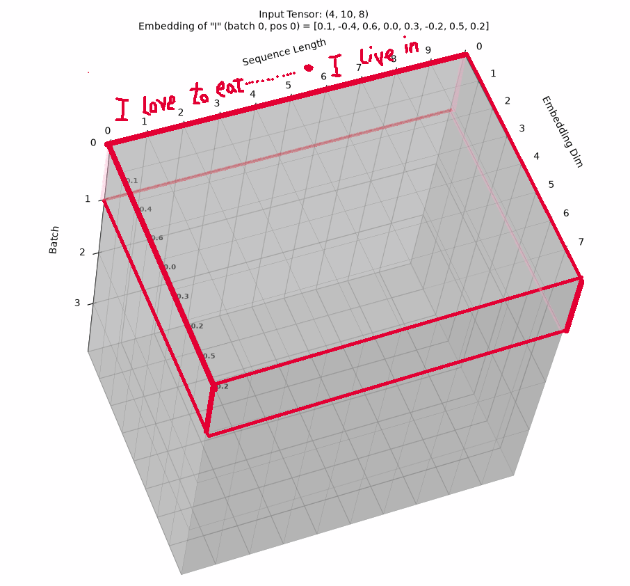
During training, we group multiple sequences together into a single batch.

A typical batch size for training a large LLM (like LLaMA or GPT) is between 1 million and 4 million tokens (yes, really!).
Since each sequence in the batch is usually 2,048 or 4,096 tokens long, a batch might contain anywhere from 256 to 2,048 individual sequences (sentences/document chunks) all packed together.

Instead of processing Sentence 1, updating the weights, then processing Sentence 2, we do this:

Pack 1,024 sequences into a single giant 3D tensor (Batch × Sequence Length × Hidden Size).
Run the Forward Pass for all 1,024 sequences at the same time (in parallel).
Calculate the Loss by averaging the prediction errors across every single token position in every single sequence in the batch.
Run Backpropagation once.
Update the weights once using the aggregated gradients from the entire batch.

Packing

During language-model pretraining, documents may be separated by an end-of-document or end-of-text token and concatenated into fixed-length token blocks.

The boundary token is sometimes also designated as the model’s end-of-sequence token, although these are conceptually different roles.

Packing reduces or eliminates padding and increases useful-token throughput. In some systems, ordinary causal attention (Causal Mask Matrix) is retained, so later documents can technically attend to earlier packed documents.
Other systems apply document-level or block-diagonal attention masks that prevent attention across document boundaries. The EOT, EOD or EOS token alone does not impose that restriction; the attention mask does.

Where padding is still used

Fine-tuning (Supervised Tuning): When you fine-tune on a specific dataset (like instruction-following data), the datasets are much smaller. Engineers usually use Dynamic Padding—they take a batch, find the longest sequence within that specific batch, and pad the shorter ones to match. This is easier to implement and still reasonably efficient.

Batching

During training, we group multiple sequences together into a single batch.

A typical batch size for training a large LLM (like LLaMA or GPT) is between 1 million and 4 million tokens (yes, really!).
Since each sequence in the batch is usually 2,048 or 4,096 tokens long, a batch might contain anywhere from 256 to 2,048 individual sequences (sentences/document chunks) all packed together.

Instead of processing Sentence 1, updating the weights, then processing Sentence 2, we do this:

Pack 1,024 sequences into a single giant 3D tensor (Batch × Sequence Length × Hidden Size).
Run the Forward Pass for all 1,024 sequences at the same time (in parallel).
Calculate the Loss by averaging the prediction errors across every single token position in every single sequence in the batch.
Run Backpropagation once.
Update the weights once using the aggregated gradients from the entire batch.

Packing while batching

During language-model pretraining, documents may be separated by an end-of-document or end-of-text token and concatenated into fixed-length token blocks.

The boundary token is sometimes also designated as the model’s end-of-sequence token, although these are conceptually different roles.

Packing reduces or eliminates padding and increases useful-token throughput. In some systems, ordinary causal attention is retained, so later documents can technically attend to earlier packed documents. Other systems apply document-level or block-diagonal attention masks that prevent attention across document boundaries. The EOT, EOD or EOS token alone does not impose that restriction; the attention mask does.

Where padding is still used

Attention

Attention is not a single number, it is a matrix;

The Complete Forward Pass Visualized

To see exactly how data moves forward through a single Attention Layer, here is the mathematical sequence from start to finish:

Projection Phase:

𝐻0 (The initial dynamic tensor built from word embeddings and positions) =$\text{Input\ Matrix\ }X\xrightarrow{\text{Forward}}\begin{cases}Q=XW_{Q}\\ K=XW_{K}\\ V=XW_{V}\end{cases}$

Core Attention Mechanism:

$A=\text{Softmax}\left(\frac{Q\cdot K^{T}}{\sqrt{d_{k}}}+M\right)$

In a single-head model, $d_{k}$ equals $d_{\text{model}}$. However, in a Multi-Head Attention model, $d_{\text{model}}$ is cleanly split across the heads:

$d_{k}=\frac{d_{\text{model}}}{\text{Number\ of\ Heads}}$

$O_{\text{raw}}=A\cdot V$

Output Projection:

$O_{\text{projected}}=O_{\text{raw}}W_{O}$
Residual and Layer Norm:

𝐻1 (The dynamic tensor outputted by Layer 1) =$\text{Layer\ Output}=\text{LayerNorm}(X+O_{\text{projected}})$

What Happens in the Backward Pass?

During training, the backward pass (backpropagation) goes in the exact opposite direction. [1, 2]

The model calculates the error (loss) at the very end.
It passes gradients backward through steps 4, 3, 2, and 1.
It uses those gradients to update the weights ($W_Q, W_K, W_V, W_O$) so the model learns better attention patterns next time. [1, 2]

$W_{O}$ stands for the Output Weight Matrix. It is a matrix of learnable parameters (weights) that the model trains during backpropagation.

Why is it Necessary? (The Multi-Head Problem)

In Multi-Head Attention, the model does not just run the attention formula once. It splits the Queries, Keys, and Values into multiple “heads” (for example, 8 or 12 heads) and runs the forward pass on all of them in parallel.

Each individual head computes its own attention output matrix.
The model concatenates (glues) all of these outputs side-by-side into one giant matrix.
This concatenated matrix is now far too wide to match the rest of the network.

The Role of $W_{O}$

The Output Matrix $W_{O}$ performs two critical jobs in the forward pass immediately after attention is calculated:

Dimension Resizing: It acts as a linear projection that shrinks the giant, concatenated multi-head matrix back down to the model’s standard hidden size (e.g., 768 or 1024 dimensions). This ensures the data fits into the next layer.
Information Mixing: It acts as a “blender.” It allows the model to mix and combine the different contextual insights learned by each individual attention head.

The Complete Multi-Head Equation

In the official Transformer architecture, this is where $W_{O}$ sits mathematically:

$\text{MultiHead}(Q,K,V)=\text{Concat}(\text{head}_{1},\text{head}_{2},\dots ,\text{head}_{h})\mathbf{W}_{\mathbf{O}}$

Without $W_{O}$, a multi-head model cannot pass its data to the next layer because the matrix dimensions would be broken.

$X$ is exactly $H_{0}$ when you are looking at the very first layer of the Transformer.

To make the math perfectly consistent across the whole network, researchers use a general symbol ($X$) for the input matrix, but its actual identity changes depending on which layer you are currently looking at:

In Layer 1: $X = H_0$ (The initial dynamic tensor built from word embeddings and positions).
In Layer 2: $X = H_1$ (The dynamic tensor outputted by Layer 1).
In Layer 3: $X = H_2$ (The dynamic tensor outputted by Layer 2).

The Generalized Formula

If you look at any arbitrary layer in the model (let’s call it Layer $l$), the projection phase during the forward path is formally written like this:

$Q=H_{l-1}W_{Q},\quad K=H_{l-1}W_{K},\quad V=H_{l-1}W_{V}$

This reveals the elegant, repeating nature of the Transformer: every single layer runs the exact same mathematical forward path, simply taking the dynamic tensor activation from the previous floor and using its own unique weight matrices to project it into a brand new set of Queries, Keys, and Values.

Gemini:

Next-Token Prediction: The model reads billions of text sequences and repeatedly guesses the next token. [1, 2]

You have an input matrix $X$, which contains the token embedding.

1. Linear Projections

Multiplying $X$ by $W_{v}$ produces the Value vectors:

$V=X\cdot W_{v}$

Multiplying $X$ by $W_{q}$ produces the Query vectors:

$Q=X\cdot W_{q}$

Multiplying $X$ by $W_{k}$ produces the Key vectors:

$K=X\cdot W_{k}$

2. Raw Attention Scores

The model calculates the raw, unmasked attention scores by checking how well every query matches every key. For a sequence of length $N$, this produces an $N \times N$ matrix:

$\text{Raw\ Scores}=\frac{Q\cdot K^{T}}{\sqrt{d_{k}}}$

(Note: $\sqrt{d_{k}}$ is the standard scaling factor used to prevent gradients from exploding. The square root of the number of dimensions. ).

3. Injecting the Causal Mask Matrix ($M$)

This is where the Causal Mask Matrix ($M$) is applied. $M$ is an $N \times N$ matrix defined as:

$M_{ij}=\begin{cases}0&\text{if\ }i\ge j\quad \text{(past\ and\ current\ tokens)}\\ -\infty &\text{if\ }i<j\quad \text{(future\ tokens)}\end{cases}$

The model adds the causal mask matrix directly to the raw attention scores:

$\text{Masked\ Scores}=\left(\frac{Q\cdot K^{T}}{\sqrt{d_{k}}}\right)+M$

Because any number added to $-\infty $ becomes $-\infty $, all future token positions in the grid are instantly driven to negative infinity. [1]

4. The Softmax Step

The model applies the Softmax function to the masked scores which are unnormalized log-probabilities (AI people call logits):

$\text{attention weights (or alignment matrix)}=\text{Softmax}\left(\left(\frac{Q\cdot K^{T}}{\sqrt{d_{k}}}\right)+M\right)$

Because $e^{-\infty} = 0$, the mathematical output of the Softmax layer forces the attention weight for all future tokens to be exactly 0 and for the previous tokens assigns a probability that is a little more for the right token

When future tokens are zeroed out, the Softmax function must still distribute a total probability sum of 1.0 across the remaining allowed tokens. [1]

Redistribution: The probability mass that would have gone to future tokens is redistributed among the past and current tokens.
Higher Scores: This mathematically inflates the final attention weights for the allowed context, often favoring the current token or relevant past context tokens

the Softmax function in this context outputs a matrix of weights rather than a single vector. [1, 2, 3, 4]

Matrix Dimensions

The variables in the equation are matrices representing an entire sequence of tokens, not individual vectors or numbers. Let $n$ represent the sequence length (number of tokens) and $d_{k}$ represent the dimension of the keys and queries. [1, 2, 3, 4, 5]

$Q$ (Query Matrix): Shape is $(n \times d_k)$
$K^{T}$ (Transposed Key Matrix): Shape is $(d_k \times n)$
$Q \cdot K^T$ (Dot Product): Shape is $(n \times n)$ [1, 2, 3, 4, 5]

How Softmax Processes the Matrix

Because $Q \cdot K^T$ results in an $(n \times n)$ matrix, the Softmax function is applied row-wise across this grid. [1, 2]

Input to Softmax: An $(n \times n)$ matrix of raw similarity scores.
Softmax Operation: Converts each row of $n$ scores into a probability distribution.
Output of Softmax: An $(n \times n)$ Attention Matrix (or alignment matrix). [1, 2, 3]

Visualizing the Result

Every single cell $(i, j)$ in the resulting matrix is a number between $0$ and $1$.

Rows ($i$): Represent the token currently looking for context.
Columns ($j$): Represent how much attention that token pays to every other token in the sequence.
Row Sum: Every individual row sums up exactly to $1$. [1]

Final Multiplication

To get the final Attention output, this $(n \times n)$ weight matrix is multiplied by the Value matrix $V$ (shape $n \times d_v$).

$\text{Shape:\ }\underbrace{(n\times n)}_{\text{Softmax\ Matrix}}\times \underbrace{(n\times d_{v})}_{V\text{\ Matrix}}=\underbrace{(n\times d_{v})}_{\text{Final\ Output\ Matrix}}$

This yields a context-rich vector of size $d_{v}$ for every single one of the $n$ tokens in your sequence simultaneously.

5. Calculating Layer Output

It multiplies these safely blocked attention scores by the Value vectors:

$\text{Layer\ Output}=\text{Attention}\cdot V$

To complete the mathematical definition of Attention, these weights must be multiplied by the Value matrix (V): [1, 2]

𝑂raw =$\text{Attention}(Q,K,V)=\text{Softmax}\left(\frac{Q\cdot K^{T}}{\sqrt{d_{k}}}+M\right)V$

Because the future tokens have an attention weight of 0, zero information from $W_{v}$ or $X$ for future words can leak into the current token’s representation.

This output passes through feed-forward networks and normalization layers.

$W_{O}$ is a matrix of static weights (parameters). The input to layer 2 is the tensor of dynamic data (activations) produced after multiplying by $W_{O}$ and passing through a few final steps. [1, 2]

Here is the exact distinction of how the data flows from Layer 1 to Layer 2:

If we look at the math, the output of the attention mechanism is a data matrix $O_{\text{raw}}$. We multiply this data by the weights $W_{O}$ to project it:

$\text{Projected\ Data}=O_{\text{raw}}\cdot W_{O}$

This “Projected Data” contains the actual token representations.

The Final Steps Before Layer 2

Before this data can enter Layer 2, a standard Transformer block passes it through two more structural components within Layer 1:

The Feed-Forward Network (FFN): The projected data is sent through a mini fully connected neural network (usually two linear layers with a GELU or ReLU activation in between). [1, 2]
Residual Connections & Layer Norm: Throughout these steps, the original inputs are added back (residual links), and the values are normalized.

Finally, the model produces a probability distribution over the entire vocabulary and predicts the next token cleanly, without cheating (looking on future tokens).

An LLM answers your question by treating it as a fill-in-the-blank exercise. It doesn’t search for the answer; it writes what it believes is the most statistically perfect continuation of your sentence, based on everything it has ever read.

An LLM doesn’t “think,” “reason,” or “look up” the answer like a search engine. Instead, it treats your entire question as the opening of a story, and its only job is to predict the very next word that should come after it. It does this over and over again, one word at a time, until the story feels complete.

Here is the step-by-step breakdown of how that works:

1. Tokenization (Turning words into math)
The LLM cannot read letters. First, it chops your question (“What is the capital of France?”) into small pieces called tokens (words or sub-words). It then converts these tokens into a list of numbers (vectors) that represent the words’ meanings and their positions in the sentence.

2. Contextualization (The “Attention” step)
The model passes your numbered question through dozens of “transformer” layers. In these layers, the model uses a mechanism called self-attention. It looks at every word in your question and measures how much it relates to every other word.

For example, in “capital of France,” it heavily links “capital” and “France” together, while ignoring “what” and “is.”
It doesn’t just look at the literal dictionary definitions; it looks at the patterns of how these words are used across the internet, books, and Wikipedia. Through this process, it builds a massive mathematical “context map” of your question.

3. The Probability Distribution (The big bet)
Now that the model has a deep mathematical understanding of your question, it reaches into its “brain”—which is essentially a massive database of billions of numerical weights (parameters) learned during training.

It calculates a probability score for every single token in its entire vocabulary (usually 50,000 to 100,000 words/pieces) to determine which one is most likely to come next.

At this exact moment, the model’s internal math looks something like this:

85% chance the next word is “Paris”
7% chance the next word is “London”
3% chance the next word is “Berlin”
0.5% chance the next word is “The”… and so on.

4. Selection and Recursion (The loop)
The model picks the token with the highest probability (or uses a bit of randomness to make it sound natural). It outputs “Paris”.

Now, the model adds “Paris” to the end of your original question. Its new input becomes:
"What is the capital of France? Paris"

It runs the entire process again, from scratch, on this new, longer sequence. Now it predicts the next token after “Paris”:

96% chance the next token is “.” (period)
3% chance it is “,”
1% chance it is “is”

It outputs “.”. The input becomes: "What is the capital of France? Paris."

It runs again. Now, it predicts there is a 99.9% chance the next token is “[End-of-Text]”, signaling that the answer is complete. It stops.

The Magic: Where does the “knowledge” come from?

This raises the obvious question: How does the math know that “Paris” has an 85% probability?

Because during its training, the LLM read billions of pages of text. It never “memorized” the fact that Paris is the capital of France. Instead, it adjusted its internal math (those billions of weights) so that whenever the pattern "capital of [Country]" appears in a prompt, the mathematical pathway that leads to "[Capital City]" fires most strongly.

The Big Catch: Why it sometimes fails

Because it is just predicting text patterns, not retrieving facts:

If you ask: “What is the capital of a country called Frants?” (misspelled), it might predict “Paris” anyway because the pattern is close, or it might hallucinate a fake city because “Frants” doesn’t match any known pattern in its training data.

Let’s use the architectural similar to a standard model like ChatGPT:

Total Attention Heads per Layer: 2
Per-Head Dimension Size: 4

with 100 layers, at first we have 100 Wq, 100 Wk, 100 Wv filled with different random numbers. Wq1 will remain a random set of numbers, not learning anything, until backpropagation are complete and Wq2 is updated and we reach to Wq1.

Following the strict rule: $\text{2 Heads} \times \text{4 Dimensions Each} = \text{8 Total Dimension Size}$. The math balances perfectly, so we can use standard square matrices without any compression tricks.

Step 1: The Input Tensor ([3, 8])

We have our 3 tokens ("I", "love", "to"). Each token is represented by exactly 8 random floating-point numbers looked up from the model’s starting vocabulary grid.

Index 0 ("I"):    [  0.1, -0.4,  0.6,  0.0,  0.3, -0.2,  0.5,  0.2 ]
Index 1 ("love"): [  0.8,  0.2, -0.1,  0.5, -0.6,  0.1,  0.0, -0.3 ]
Index 2 ("to"):   [ -0.3,  0.7,  0.2, -0.5,  0.4,  0.9, -0.1,  0.6 ]

Use code with caution.

Step 2: The Model’s Brain (The 8 × 8 Permanent Weight Matrices)

Because our embedding size is 8, the model’s permanent internal weight layers are perfectly square grids of 8 rows by 8 columns.

The GPU multiplies our input tensor by these three permanent parameter grids to generate three new full-sized matrices of shape [3, 8]:

Matrix A: Reassigned numbers that will act as the Seekers
Matrix B: Reassigned numbers that will act as the Labels
Matrix C: Reassigned numbers that will act as the Meanings

the exact formula is $Q = X W_q$.

In this equation, $X$ represents your input tensor, and $W_{q}$ represents the permanent Query weight matrix.

1. Shape the Input

Row count: $3$ tokens within your current sequence.
Column count: $8$ dimensions for the vector embeddings.
Tensor shape: $X$ uses a shape of $[3, 8]$.

2. Configure the Weights

Row size: $8$ rows matching input dimensions.
Column size: $8$ columns matching target projection dimensions.
Tensor shape: $W_{q}$ features a grid of $[8, 8]$.

3. Multiply the Matrices

Operation rule: Matrix multiplication targets inner dimensions.
Dimension cancellation: The inner dimensions of $8$ resolve.
Output shape: $Q$ maintains a final shape of $[3, 8]$.

The mathematical operation to generate your Query matrix is $Q = X W_q$, which multiplies your $[3, 8]$ input sequence by the permanent $[8, 8]$ weight grid to yield the final $[3, 8]$ Seeker matrix.T

The Query vector ($Q$) searches through all the available Keys ($K$) to see which tokens have the information it needs

Let’s assume the random matrix multiplications output these numbers:

Matrix A (The Seeker Vectors==Query Vector)

Index 0 ("I"):    [  0.5, -0.2,  0.1,  0.4,   0.2,  0.7, -0.1,  0.0 ]
Index 1 ("love"): [ -0.1,  0.6,  0.3, -0.3,   0.0,  0.4,  0.8,  0.2 ]
Index 2 ("to"):   [  0.4,  0.2, -0.5,  0.1,   0.6, -0.2,  0.3,  0.5 ] <-- We will trace this row

Matrix B (The Label Vectors==Key Vector)

Index 0 ("I"):    [  0.2,  0.8, -0.1,  0.3,   0.5,  0.1,  0.0,  0.4 ]
Index 1 ("love"): [  0.6, -0.4,  0.5,  0.0,  -0.2,  0.9,  0.3,  0.1 ]
Index 2 ("to"):   [ -0.2,  0.5,  0.1,  0.7,   0.4, -0.1,  0.6,  0.0 ]

Matrix C (The Meaning Vectors==Value Vector)

Index 0 ("I"):    [  1.0, -0.5,  0.2,  0.6,   0.0,  0.8, -0.3,  1.1 ]
Index 1 ("love"): [  0.0,  1.2, -0.4,  0.1,   1.5, -0.2,  0.7,  0.0 ]
Index 2 ("to"):   [  0.4,  0.1,  0.8, -0.3,  -0.5,  0.6,  0.2,  0.9 ]

Step 3: The Head Slicing (4 Columns per Head)

The GPU now executes the slicing hyperparameter. It takes those 8-column wide matrices and slices them cleanly down the middle into 2 independent heads, each getting exactly 4 columns.

text

                  HEAD 1 (Columns 0, 1, 2, 3)             HEAD 2 (Columns 4, 5, 6, 7)
Seeker Slices:    "I"   : [  0.5, -0.2,  0.1,  0.4 ]      "I"   : [  0.2,  0.7, -0.1,  0.0 ]
                  "love": [ -0.1,  0.6,  0.3, -0.3 ]      "love": [  0.0,  0.4,  0.8,  0.2 ]
                  "to"  : [  0.4,  0.2, -0.5,  0.1 ]      "to"  : [  0.6, -0.2,  0.3,  0.5 ]

Label Slices:     "I"   : [  0.2,  0.8, -0.1,  0.3 ]      "I"   : [  0.5,  0.1,  0.0,  0.4 ]
                  "love": [  0.6, -0.4,  0.5,  0.0 ]      "love": [ -0.2,  0.9,  0.3,  0.1 ]
                  "to"  : [ -0.2,  0.5,  0.1,  0.7 ]      "to"  : [  0.4, -0.1,  0.6,  0.0 ]

Meaning Slices:   "I"   : [  1.0, -0.5,  0.2,  0.6 ]      "I"   : [  0.0,  0.8, -0.3,  1.1 ]
                  "love": [  0.0,  1.2, -0.4,  0.1 ]      "love": [  1.5, -0.2,  0.7,  0.0 ]
                  "to"  : [  0.4,  0.1,  0.8, -0.3 ]      "to"  : [ -0.5,  0.6,  0.2,  0.9 ]

Use code with caution.

Step 4: Tracing Head 1’s Math for Index 2 (“to”)

Let’s see how the GPU core running Head 1 calculates relationship scores for Index 2. It takes the Seeker Slice for “to” [0.4, 0.2, -0.5, 0.1] and dot-multiplies it (cross-multiply and sum) against all Labels:

vs Index 0 Label (“I”): [0.2, 0.8, -0.1, 0.3]

$\text{Score}=(0.4\times 0.2)+(0.2\times 0.8)+(-0.5\times -0.1)+(0.1\times 0.3)=0.08+0.16+0.05+0.03=\mathbf{0.32}$
vs Index 1 Label (“love”): [0.6, -0.4, 0.5, 0.0]

$\text{Score}=(0.4\times 0.6)+(0.2\times -0.4)+(-0.5\times 0.5)+(0.1\times 0.0)=0.24-0.08-0.25+0.00=\mathbf{-0.09}$
vs Index 2 Label (“to”): [-0.2, 0.5, 0.1, 0.7]

$\text{Score}=(0.4\times -0.2)+(0.2\times 0.5)+(-0.5\times 0.1)+(0.1\times 0.7)=-0.08+0.10-0.05+0.07=\mathbf{0.04}$

The GPU computes all rows simultaneously, generating Head 1’s raw matching grid:

                LABELS (Head 1)
               "I"     "love"    "to"
   "I"      [  0.15     0.28     0.02  ]
SEEKERS     [  0.54    -0.12     0.41  ]
   "to"     [  0.32    -0.09     0.04  ] <-- Our calculated row sitting at Index 2

Use code with caution.

Step 5: Causal Mask and Softmax (Enforcing the Timeline)

The causal mask matrix instantly overwrites future positions with $-\infty $. Then, Softmax converts the row vectors into clean focus percentages that sum up to 1.0. For our row at Index 2, the math yields:

               SOFTMAX PERCENTAGES (Head 1)
                 "I"     "love"    "to"
        "to"   [ 0.40     0.26     0.34 ]  --> 40% focus on "I", 26% on "love", 34% on "to"

Use code with caution.

Step 6: Blending Head 1’s Meanings

The GPU core blends Head 1’s Meaning Slices together using those focus percentages:

$\text{Head\ 1\ Output}_{2}=(0.40\times \text{Meaning}_{0})+(0.26\times \text{Meaning}_{1})+(0.34\times \text{Meaning}_{2})$

$\text{Head\ 1\ Output}_{2}=0.40\times [1.0,-0.5,0.2,0.6]+0.26\times [0.0,1.2,-0.4,0.1]+0.34\times [0.4,0.1,0.8,-0.3]$

Let’s execute the addition coordinate-by-coordinate:

Dim 0: $(0.40 \times 1.0) + (0.26 \times 0.0) + (0.34 \times 0.4) = 0.40 + 0.00 + 0.136 = \mathbf{0.536}$
Dim 1: $(0.40 \times -0.5) + (0.26 \times 1.2) + (0.34 \times 0.1) = -0.20 + 0.312 + 0.034 = \mathbf{0.146}$
Dim 2: $(0.40 \times 0.2) + (0.26 \times -0.4) + (0.34 \times 0.8) = 0.08 – 0.104 + 0.272 = \mathbf{0.248}$
Dim 3: $(0.40 \times 0.6) + (0.26 \times 0.1) + (0.34 \times -0.3) = 0.24 + 0.026 – 0.102 = \mathbf{0.164}$

$\text{Head\ 1\ Output\ Vector}_{2}=[0.536,0.146,0.248,0.164]$

Step 7: Concatenation Stitching (Rebuilding the 8 Highway)

While Head 1 calculated that 4-dimensional array for Index 2, Head 2 was running its own slice data on a separate core and produced its own 4-dimensional vector—let’s say it calculated [-0.088, 0.412, 0.901, -0.334].

To exit the attention mechanism, the model strings the two halves together side-by-side:

text

       Head 1 Output Slice                  Head 2 Output Slice
  [ 0.536, 0.146, 0.248, 0.164 ]     +     [ -0.088, 0.412, 0.901, -0.334 ]

                                     =

                        THE STITCHED RESULT
  [ 0.536, 0.146, 0.248, 0.164, -0.088, 0.412, 0.901, -0.334 ]

This 8-dimensional array is written directly back into Index 2 of the layer’s final output tensor. Because the horizontal slicing rule matches perfectly ($\text{2 heads} \times \text{4 dimensions} = \text{8}$), the output is already the exact right width to hit the network’s main highway without needing an extra projection matrix step.

Now that you have traced the cleanest possible version of the attention pipeline, would you like to see how multi-head attention differs from the next major block in the layer—the Feed-Forward Network (FFN)?

During training with transformer model, we never feed just a 1D tensor. We wrap it into a 2D tensor (a matrix) of shape [Batch_Size, Sequence_Length]—which is basically an array of arrays—so the GPU can process all your 4 sentences at the exact same time in parallel.

The placement of words in that 4,000-dimensional space is entirely unsupervised (or more precisely, self-supervised).

Here is the radical reality: No human teacher, no dictionary, and no labeled dataset tells the model where to place “pizza” or “burgers.” The model figures out the coordinates entirely by itself, simply by reading billions of sentences.

Here is exactly how this unsupervised placement happens in practice:

1. The “Gravity” of Context (The Distributional Hypothesis)

The model operates on a single, ruthless rule: “Words that appear in the exact same contexts must be placed near each other.”

When the model sees "I love to eat" → "pizza" (Sentence 1) and "I love to eat" → "burgers" (Sentence 2), it doesn’t “know” they are foods.
Instead, the math (backpropagation) looks at the error for both predictions and physically pulls the vectors for “pizza” and “burgers” closer together in the 4,000-D space, because they keep showing up in identical environments.
This is called the Distributional Hypothesis: “You shall know a word by the company it keeps.”

2. How the 4,000 Dimensions get “Carved Up”

Because no one is labeling the data, the model uses those 4,000 dimensions as free parameters to encode any pattern it finds useful.

Over time, the unsupervised process naturally dedicates different dimensions to different hidden features:

Dimension #1,203 might become the “Italian food” axis (pizza and pasta have high values here, burgers don’t).
Dimension #3,401 might become the “Fast food” axis (burgers and fries cluster here, pizza has a mid-range value).
Dimension #2,800 might become the “edible noun” axis, separating all foods from prepositions like “on” and “top”.

The model invents these categories on its own. It doesn’t name them; it just mathematically organizes them to minimize future prediction errors.

3. The “Cold Start” (Initial Randomness vs. Final Order)

To be perfectly accurate: The initial placement is random.
Before training, the 4,000 numbers for “pizza” are just random noise (e.g., [0.02, -0.55, 0.31, ...]).

The unsupervised training process is like a giant, 4,000-dimensional game of Gravity and Repulsion:

When two words are interchangeable in a sentence, gradients pull their coordinates together.
When two words never share contexts (e.g., “pizza” and “therefore”), they drift far apart.
After training on your heap (and billions of other sentences), this random noise self-organizes into a beautiful, intricate, geometric map of human language—without a single human telling the model what a “noun” or a “verb” is.

4. The Crucial Modern Twist: Subword Unsupervision

Because modern models use BPE (Byte-Pair Encoding), this unsupervised placement even happens for fake, non-words. If your tokenizer splits "ketchup" into ["ket", "chup"], the model unsupervisedly learns that when "ket" is immediately followed by "chup", their combined vector should point to the same region as "mustard" and "relish". It learns that these fragments belong together purely from repetitive patterns in the raw heap.

To sum it up in one sentence:
The 4,000 numbers are not “translated” from a dictionary; they are forged by the model observing millions of unsupervised permutations. The human just provides the raw heap; the AI teaches itself the map. This is why LLMs can work for any language—they don’t need a pre-built grammar book, they just need the raw, unlabeled text.

Here is what is actually happening inside the computer at that exact millisecond:

Step 1: The Prediction (The Guesses)

The model has processed "I love to eat". In its 4,000-dimensional space, it does the math and outputs a probability distribution across the entire 50,000-word vocabulary.

It looks like this:

Probability of "pizza" = 0.4 (40% sure)
Probability of "burgers" = 0.3 (30% sure)
Probability of "sushi" = 0.05
Probability of "rocks" = 0.001
…and so on, with all probabilities adding up to exactly 1.0.

Step 2: The Target (The “Perfect” Answer)

The computer knows the correct next word from your heap is "pizza".
But the computer can’t just say “Good job” or “Bad job”. It needs a pure number to do math with.

So, it creates a “perfect” target vector called a One-Hot Encoding:

"pizza" gets a score of 1.0 (100% correct).
Every single other word in the entire 50,000 vocabulary (including “burgers”) gets a score of 0.0.

Step 3: The Loss (Measuring “How Wrong” the guess is)

Now we have two numbers for “pizza”:
The model guessed 0.4, but the target says it should have been 1.0.

The Loss Function (often called Cross-Entropy Loss, though here simplified to a basic subtraction) calculates the error:

Loss = Target - Prediction
Loss = 1.0 - 0.4 = 0.6

That 0.6 is the “Magnitude of Wrongness.”
If the model had guessed 0.9, the loss would have been 0.1 (a tiny error). If it had guessed 0.0, the loss would have been 1.0 (a massive error).

Step 4: The Derivative (The “Direction” to turn the dials)

This is the magic step. The model doesn’t just care that it was wrong; it needs to know which way to turn the dials to make that 0.6 smaller next time.

The derivative is simply the mathematical “slope” of that error.

Because the error is positive (1.0 – 0.4 = +0.6), the slope tells the model: “Hey, the number for ‘pizza’ is too low. You need to increase it.”
If the error were negative (meaning it guessed too high), the derivative would say: “Turn the dials the opposite way to decrease it.”
The derivative also tells us how hard to turn: a big error (0.6) gives a steep slope, meaning we turn the dials aggressively. A tiny error gives a gentle slope, meaning we make tiny micro-adjustments.

Step 5: Tweaking the Weights (Turning the Dials)

Now we get to the weights—these are the 7+ billion internal dials (numbers) inside the neural network.

The computer takes that derivative (slope) and multiplies it by a tiny number called the Learning Rate (e.g., 0.001).

It then subtracts this value from every single weight that contributed to the prediction of “pizza”.
The weights that pushed the model toward “pizza” get turned up slightly (so next time, “pizza” scores higher).
The weights that pushed the model toward “burgers” get turned down slightly (so next time, “burgers” steals less attention in this specific context).

A crucial correction to the simplified math:

In actual modern AI, we don’t simply do 1.0 - 0.4 = 0.6.
We use Negative Log Likelihood, which calculates -log(0.4) = 0.91.

Why? Because if the model guessed 0.01 (1% confidence), -log(0.01) equals 2.0—a huge penalty. If it guessed 0.99, -log(0.99) equals 0.01—a tiny penalty. The logarithmic loss punishes overconfidence harshly and rewards high confidence exponentially. But the core concept is exactly what I described: Compare the prediction to the target, get a single “error” number, find its slope, and push that slope backward through the network to turn the dials so that next time, the error number is smaller.

To sum it up like a human coach:
The model guessed “pizza” with 40% confidence. The coach (loss function) says, “You should have been 100% sure. You missed by 60%.” The coach calculates the exact direction to push the player’s arms (derivative) so that next time they swing 60% less wrong. That push flows backward through the entire network (backpropagation), adjusting billions of internal dials by microscopic amounts, making the model slightly smarter for the next batch of sentences.

That 0.4 does not magically appear. It is the result of a specific mathematical “squeeze” function called Softmax.

Here is exactly where the 0.4 comes from, step-by-step:

Step 1: The Raw Output (Logits)

The output of a transformer before the softmax layer consists of unnormalized log-probabilities which AI people call logits.

After the model processes "I love to eat" through all its billions of calculations, the very last layer outputs a giant list of raw, unbounded numbers which we call choose to call Logits.

For the sake of this example, let’s say the model outputs a raw score for just these two words:

Raw score for "pizza" = 2.5
Raw score for "burgers" = 2.2

Notice a problem? These numbers are not probabilities. They are just arbitrary floating-point numbers. They could be -5.0 or 15.0. They don’t sum to 1.0, and they don’t tell you a “percentage chance” yet.

Step 2: The Softmax Converts Unnormalized log-probabilities to Probabilities

The model immediately passes that giant list of raw scores through a function called Softmax.

The Softmax function does two specific things to those raw numbers:

It exponentiates them (raises Euler’s number *e*, roughly 2.718, to the power of the raw score). This makes all numbers positive and amplifies the gap between them.
It divides each exponentiated score by the sum of all exponentiated scores across the entire 50,000-word vocabulary. This forces every single output to land strictly between 0.0 and 1.0, and forces all of them to add up to exactly 1.0.

Step 3: The Math in Action

Let’s do the math for just “pizza” and “burgers” to see how 0.4 and 0.3 appear.

The raw scores (logits) were:

logit(pizza) = 2.5
logit(burgers) = 2.2

First, exponentiate them:

e^(2.5) = 12.18
e^(2.2) = 9.02

Second, divide each by the total sum (12.18 + 9.02 = 21.20):

Probability of "pizza" = 12.18 / 21.20 = 0.57
Probability of "burgers" = 9.02 / 21.20 = 0.42

(Note: In my original simplified example, I used 0.4 and 0.3 just to make the subtraction easy. The real math above gives 0.57 and 0.42.)

Why does the model output 0.4 for pizza and 0.3 for burgers specifically?

Because the neural network looked at the context "I love to eat" and through all its internal matrix multiplications, it calculated:

A logit of 2.5 for “pizza”
A logit of 2.2 for “burgers”

Why is the logit for pizza slightly higher (2.5 vs 2.2)?
Because during training, the model saw "I love to eat pizza" in Sentence 1, and "I love to eat burgers" in Sentence 2. When the two gradients pulled in opposite directions, the optimizer settled on an equilibrium where “pizza” gets a slightly stronger weight connection in that specific context than “burgers” does.

So, the 0.4 you asked about is literally just:

Softmax(2.5) = 0.57 (or roughly ~0.4 in a larger vocabulary where millions of other words are also stealing tiny fractions of that probability mass).

In Summary: The exact pipeline to get 0.4

Step	Data	What happened?
1. Input	`"I love to eat"`	Passed through the Transformer layers.
2. Raw Math	Logit for `"pizza"` = 2.5	The network’s internal weights produced a raw score.
3. Softmax	`e^2.5 / (e^2.5 + e^2.2 + ...)`	Squeezed the raw score into a percentage.
4. Output	Probability = 0.4 (or 0.57)	The final, interpretable “confidence” number.

So, to directly answer: 0.4 comes from the Softmax function violently compressing the network’s arbitrary raw math (which could be anything from -infinity to +infinity) into a clean, readable probability that sums to 100% across all guesses.

The embedding for the word “pizza” is 4,000 numbers.
The hidden state for the context “I love to eat” is 4,000 numbers.
But the logit for “pizza” is exactly 1 single number (e.g., 2.5).

Here is exactly how we get from the 4,000 numbers down to that single logit number:

Step 1: The Hidden State (4,000 numbers)

When the model processes "I love to eat", the final Transformer layer outputs a single hidden state vector for the last token ("eat").
This vector is 4,000 numbers long:
[0.5, -1.2, 0.8, 2.1, -0.3, ...] (4,000 of them).

This 4,000-number vector is the model’s “mathematical understanding” of the entire phrase "I love to eat".

Step 2: The Output Weight Matrix (50,000 × 4,000)

The model has a giant final layer called the LM Head (Language Model Head). This is just a massive matrix of weights.

It has 50,000 rows (one for every word in the vocabulary).
It has 4,000 columns (to match the hidden state size).

Inside this matrix, the row dedicated to the word "pizza" contains exactly 4,000 numbers (its own unique weights).

Step 3: The Dot Product (Getting 1 number)

To get the raw logit for "pizza", the computer performs a Dot Product (element-wise multiplication and summation) between:

The 4,000-number hidden state (from the phrase)
The 4,000-number weight row for "pizza"

The math looks like this:
(0.5 * 0.1) + (-1.2 * 0.3) + (0.8 * -0.5) + (2.1 * 0.9) + ... (4,000 times)

When you multiply and add all 4,000 pairs together, the result collapses into a single number.
That single number is the logit for “pizza” (let’s say it equals 2.5).

Step 4: Repeat for all words

The computer does this exact same dot product for every single row in the 50,000 × 4,000 matrix:

Hidden state (4k) × Weight row for “pizza” (4k) = Logit for “pizza” = 2.5
Hidden state (4k) × Weight row for “burgers” (4k) = Logit for “burgers” = 2.2
Hidden state (4k) × Weight row for “sushi” (4k) = Logit for “sushi” = 1.1
…and so on, 50,000 (size of vocabulary) times.

The final output is a 1D tensor (array) of 50,000 logits—one single number per word in the vocabulary.

The Big Picture Summary:

What it is	Shape (Size)	What it represents
Hidden State (the context)	4,000 numbers	The model’s mathematical understanding of `"I love to eat"`.
Weight Row for “pizza”	4,000 numbers	The model’s stored “profile” for what contexts trigger the word “pizza”.
The Math	Dot Product (4k × 4k)	Comparing the context against the profile of “pizza”.
Logit for “pizza”	1 number (2.5)	How strongly the context matches “pizza” before turning it into a probability.
All Logits	50,000 numbers	Raw scores for every word in the vocabulary.
Softmax Output	50,000 numbers (probabilities)	The 50,000 logits squeezed into percentages (e.g., 0.4 for pizza).

In natural language processing, the specific sequences “I”, “I love”, “I love to”, and “I love to eat” are called prefixes or antecedents.

When referring to the vectors themselves at those specific tensor indices, engineers call them causally contextualized token representations or simply prefix representations.

Loss and Gradients in a Neural Network

The loss is calculated at the final output layer. However, gradients are calculated for every trainable parameter in every layer in the backward propagation, all the way back through the network.

To understand why, we must separate the calculation of the loss from the distribution of the gradient.

1. Where Is the Loss Calculated?

The loss is calculated at the end of the network, after the model produces its final output.

For next-token prediction, the model compares:

Its predicted probability distribution over the vocabulary
The ground-truth target token

This comparison is usually performed using cross-entropy loss.

Crucially: You do not normally calculate a separate loss for Layer 3, Layer 4, or each attention head. The network produces one overall loss value for the forward pass or training batch.

Important qualification: During standard language-model training, cross-entropy is usually calculated at every predicted token position in the training sequence. These token-level losses are then summed or averaged to produce the overall loss for the training step.

In a sequence of 2,048 tokens, the model makes a prediction at every single token position (except the first one, because there is no previous token to predict it).

So yes, cross-entropy is calculated 2,047 times for that single sequence—once for each predicted position.

2. Where Are the Gradients Calculated?

This is where backpropagation enters the process.

Although the overall loss is produced at the output, calculus—particularly the chain rule—is used to distribute responsibility for that loss backward through every operation performed by the model.

Therefore, gradients are calculated for every trainable parameter:

\[ \frac{\partial L}{\partial W} \]

They are calculated in reverse order:

The gradient is calculated for the final linear or unembedding layer.

“`

The gradient is passed backward through the final normalization operation.
It is passed backward through the final feed-forward network.
It enters the final attention layer, where gradients are calculated for parameters such as:

\[ \frac{\partial L}{\partial W_Q}, \qquad \frac{\partial L}{\partial W_K}, \qquad \frac{\partial L}{\partial W_V}, \qquad \frac{\partial L}{\partial W_O} \]
The gradient passes through the residual connections and continues into the preceding transformer layer.
This process repeats through every transformer layer, from Layer $N$ back to Layer 1.
Finally, gradients are calculated for the input-token embedding matrix and, when applicable, positional embeddings.

“`

Thus, every trainable matrix receives its own gradient, but all these gradients ultimately originate from the same overall loss.

The Train Analogy

Imagine a 100-car train representing a 100-layer neural network.

The train moves forward through all 100 layers.

“`

The loss is evaluated only after the final car reaches the destination and the conductor determines how far the train is from the correct destination.
The conductor then sends a message backward through the train.
Car 100 receives the message and determines how its own actions contributed to the error.
It passes an appropriately transformed message to Car 99.
Car 99 determines its own contribution and passes the message farther backward.
This continues until the signal reaches Car 1.

“`

Every car calculates its own adjustment, but all the adjustments originate from the error measured at the final destination.

The Mathematical Reality: The Chain Rule

Suppose the network contains layers $1$ through $N$. The gradient for a weight matrix in an early layer is calculated by multiplying the relevant derivatives along the entire computational path:

\[ \frac{\partial L}{\partial W_1} = \frac{\partial L}{\partial H_N} \cdot \frac{\partial H_N}{\partial H_{N-1}} \cdot \frac{\partial H_{N-1}}{\partial H_{N-2}} \cdots \frac{\partial H_2}{\partial H_1} \cdot \frac{\partial H_1}{\partial W_1} \]

Here:

$L$ is the loss.
$H_i$ is the output or hidden state of Layer $i$.
$W_1$ is a trainable parameter matrix in Layer 1.

The gradient for Layer 1 therefore contains the loss gradient multiplied by the derivatives of all the later operations.

The loss is not recalculated at Layer 1. Instead, information about how Layer 1 affected the loss is mathematically propagated backward.

How This Applies to the Value Matrix

In an attention layer, the value vectors are calculated as:

\[ V = XW_V \]

During backpropagation, the model calculates:

\[ \frac{\partial L}{\partial W_V} \]

Using the chain rule, this gradient depends on:

How $W_V$ changed the value vectors $V$
How the value vectors changed the attention output
How the attention output changed later hidden states
How those hidden states changed the final logits
How the logits changed the loss

Therefore, $W_V$ receives a specific gradient representing how changing it would have changed the final loss.

Residual Connections

Transformer layers contain residual connections. A simplified residual operation is:

\[ H_{\text{out}} = H_{\text{in}} + F(H_{\text{in}}) \]

During backpropagation, the gradient can travel through both paths:

The direct residual path
The transformed path through $F$

This provides a relatively direct route for gradient information and helps reduce the vanishing-gradient problem in deep transformer networks.

Auxiliary Losses

Some neural-network architectures use auxiliary losses, also called:

Intermediate losses
Deep-supervision losses
Router losses in mixture-of-experts models
Regularization losses

For example, a model might calculate additional loss terms at intermediate layers:

\[ L_{\text{total}} = L_{\text{final}} + \lambda_1 L_{\text{auxiliary-1}} + \lambda_2 L_{\text{auxiliary-2}} \]

The coefficients $\lambda_1$ and $\lambda_2$ determine how strongly the auxiliary losses influence training.

Auxiliary losses may be introduced to:

Improve gradient flow
Encourage useful intermediate representations
Balance expert utilization in mixture-of-experts models
Stabilize or accelerate training

However, the basic transformer-training principle remains the same: the primary language-model loss is produced from the model’s output predictions, and backpropagation calculates gradients for all trainable parameters that contributed to those predictions.

Summary Table

“““

Component	Where Is It Calculated?	How Often?
Token-level loss	At each predicted token position, using the final output logits	Once for each target-token position
Overall training loss	By aggregating the token-level losses, usually through a mean or sum	One overall value per training step or batch
Gradients for $W_Q$, $W_K$, $W_V$, and $W_O$	During backpropagation in every attention layer	One gradient tensor for every trainable parameter tensor
Feed-forward-network gradients	During backpropagation in every transformer layer	One gradient tensor for every trainable parameter tensor
Embedding gradients	At the bottom of the backpropagation process	Once per training step for embeddings used in the batch
Parameter updates	After backpropagation, when the optimizer uses the gradients	Normally once per optimizer step

Core Principle

The loss measures the final prediction error. Backpropagation determines how every trainable parameter contributed to that error.

The loss does not need to be recalculated separately inside every layer. Through the chain rule, the single computational graph connects the output loss to all parameters that influenced it, allowing each parameter to receive its own unique gradient.