Estimators for a population's parameters

Finding the best estimate for distribution of the population is done by maximum likelihood method. but the parameters that lead to this best distribution are sometimes biased estimators of the paraters themselves.

The method of Maximum Likelihood tries to find estimators for population parameters that create a distribution that maximizes the likelihood of observations statistics.

In maximum likelihood method, we choose the P1,P2, Pn parameteres of the population which maximize the likelihood of s1,s2,s3 statistics of samples condistional to p1,p2,p3 being the parameters of the population (Wackerly, D., Mendenhall, W., & Scheaffer, R. L. , 2001, p.449)

Continuous random variables X₁, …, X_n are all statistically independent from each other if and only if their joint density function can be factored as:

$f_{X_1,\dots,X_n}(x_1,\ldots,x_n) = f_{X_1}(x_1)\cdots f_{X_n}(x_n).$

This means that the COV(Xi,Xj)=0 Johnson, R. A., & Wichern, D. W. 2007, p. 69)

Suppose there is a sample x₁, x₂, …, x_n of n independent and identically distributed (iid) observations, coming from a distribution with an unknown probability distribution function pdf ƒ₀(·). It is however surmised that the function ƒ₀ belongs to a certain family of distributions {?ƒ(·|?), ? ? ??}, called the parametric model, so that ƒ₀ = ƒ(·|?₀). The value ?₀ is unknown and is referred to as the “true value” of the parameter. It is desirable to find some estimator $\scriptstyle\hat\theta$ which would be as close to the true value ?₀ as possible. Both the observed variables x_i and the parameter ? can be vectors.

To use the method of maximum likelihood, one first specifies the joint density function for all observations. For an iid sample this joint density function will be

$f(x_1,x_2,\ldots,x_n\;|\;\theta) = f(x_1|\theta)\cdot f(x_2|\theta)\cdots f(x_n|\theta).$

Now we look at this function from a different perspective by considering the observed values x₁, x₂, …, x_n to be fixed “parameters” of this function, whereas ? will be the function’s variable and allowed to vary freely.

MLE was first suggested by Fisher in 1920s. A MLE estimate is the same whether we maximize the likelihood or the log-likelihood function, since log is a monotone funstion. In many situations we maximize the log of the likelihood since log converts multiplications to additions which are easier to work with (Devore, P. J. L. , 2007, p. 245).

=============================================================================

This example is from wikipedia:http://en.wikipedia.org/wiki/Maximum_likelihood#Continuous_distribution.2C_continuous_parameter_space

Continuous distribution, continuous parameter space

For the normal distribution $\mathcal{N}(\mu, \sigma^2)$ which has probability density function

$f(x\mid \mu,\sigma^2) = \frac{1}{\sqrt{2\pi}\ \sigma\ } \exp{\left(-\frac {(x-\mu)^2}{2\sigma^2} \right)},$

the corresponding probability density function for a sample of n independent identically distributed normal random variables (the likelihood) is

$f(x_1,\ldots,x_n \mid \mu,\sigma^2) = \prod_{i=1}^{n} f( x_{i}\mid \mu, \sigma^2) = \left( \frac{1}{2\pi\sigma^2} \right)^{n/2} \exp\left( -\frac{ \sum_{i=1}^{n}(x_i-\mu)^2}{2\sigma^2}\right),$

or more conveniently:

$f(x_1,\ldots,x_n \mid \mu,\sigma^2) = \left( \frac{1}{2\pi\sigma^2} \right)^{n/2} \exp\left(-\frac{ \sum_{i=1}^{n}(x_i-\bar{x})^2+n(\bar{x}-\mu)^2}{2\sigma^2}\right),$

where $\bar{x}$ is the sample mean.

This family of distributions has two parameters: ? = (?, ?), so we maximize the likelihood, $\mathcal{L} (\mu,\sigma) = f(x_1,\ldots,x_n \mid \mu, \sigma)$ , over both parameters simultaneously, or if possible, individually.

Since the logarithm is a continuous strictly increasing function over the range of the likelihood, the values which maximize the likelihood will also maximize its logarithm. Since maximizing the logarithm often requires simpler algebra, it is the logarithm which is maximized below. (Note: the log-likelihood is closely related to information entropy and Fisher information.)

$\begin{align} 0 & = \frac{\partial}{\partial \mu} \log \left( \left( \frac{1}{2\pi\sigma^2} \right)^{n/2} \exp\left(-\frac{ \sum_{i=1}^{n}(x_i-\bar{x})^2+n(\bar{x}-\mu)^2}{2\sigma^2}\right) \right) \\[6pt] & = \frac{\partial}{\partial \mu} \left( \log\left( \frac{1}{2\pi\sigma^2} \right)^{n/2} - \frac{ \sum_{i=1}^{n}(x_i-\bar{x})^2+n(\bar{x}-\mu)^2}{2\sigma^2} \right) \\[6pt] & = 0 - \frac{-2n(\bar{x}-\mu)}{2\sigma^2} \end{align}$

which is solved by

$\hat\mu = \bar{x} = \sum^n_{i=1}x_i/n.$

This is indeed the maximum of the function since it is the only turning point in ? and the second derivative is strictly less than zero.

An estimator is said to be unbiased if its bias is equal to zero for all values of parameter ?.

That is, we assume that our data follows some unknown distribution P(x | ?) (where ? is a fixed constant that is part of this distribution, but is unknown), and then we construct some estimator $\hat\theta$ that maps observed data to values that we hope are close to ?. Then the bias of this estimator is defined to be

$\operatorname{Bias}[\,\hat\theta\,] = \operatorname{E}[\,\hat{\theta}\,]-\theta = \operatorname{E}[\, \hat\theta - \theta \,],$

where E[ ] denotes expected value over the distribution P(x | ?), i.e. averaging over all possible observations x.

We can show that expected value is equal to the parameter ? of the given distribution, http://www.google.ca/url?sa=t&source=web&cd=2&ved=0CB4QFjAB&url=http%3A%2F%2Fclassweb.gmu.edu%2Ftkeller%2FHANDOUTS%2FHandout6.pdf&ei=O4pATsOwF8bSiALQwY3JBQ&usg=AFQjCNHy14oE99pDSgeMQmm_R3qks3oIGA&sig2=SpONA9WK-OOa9qneipefvA

$E \left[ \widehat\mu \right] = \mu, \,$

which means that the maximum-likelihood estimator $\widehat\mu$ is unbiased.

Let X1, X2, X3, …, Xn be a simple random sample from a population with mean ?.

E(Xbar)
= E(1/n ? Xi)
= 1/n * E(?Xi)

expectation is a linear operator so we can take the sum out side of the argurement

= 1/n * ? E(Xi)

there are n terms in the sum and the E(Xi) is the same for all i

= 1/n * nE(Xi)
= E(Xi)

E(Xbar) = ?

since E(Xbar) = ?, Xbar is an unbiased estimator for the populaiton mean ?.

=================================================================

If we differentiate the log likelihood with respect to ? and equate to zero:

$\begin{align} 0 & = \frac{\partial}{\partial \sigma} \log \left( \left( \frac{1}{2\pi\sigma^2} \right)^{n/2} \exp\left(-\frac{ \sum_{i=1}^{n}(x_i-\bar{x})^2+n(\bar{x}-\mu)^2}{2\sigma^2}\right) \right) \\[6pt] & = \frac{\partial}{\partial \sigma} \left( \frac{n}{2}\log\left( \frac{1}{2\pi\sigma^2} \right) - \frac{ \sum_{i=1}^{n}(x_i-\bar{x})^2+n(\bar{x}-\mu)^2}{2\sigma^2} \right) \\[6pt] & = -\frac{n}{\sigma} + \frac{ \sum_{i=1}^{n}(x_i-\bar{x})^2+n(\bar{x}-\mu)^2}{\sigma^3} \end{align}$

the solution is:

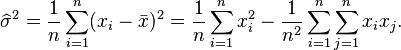
$\widehat\sigma^2 = \sum_{i=1}^n(x_i-\widehat{\mu})^2/n.$

================================

We can show that this is a biased estimator 🙁

Inserting $\widehat\mu$ we obtain

$\widehat\sigma^2 = \frac{1}{n} \sum_{i=1}^{n} (x_{i} - \bar{x})^2 = \frac{1}{n}\sum_{i=1}^n x_i^2 -\frac{1}{n^2}\sum_{i=1}^n\sum_{j=1}^n x_i x_j.$

To calculate its expected value, it is convenient to rewrite the expression in terms of zero-mean random variables (statistical error) $\delta_i \equiv \mu - x_i$ . Expressing the estimate in these variables yields

$\widehat\sigma^2 = \frac{1}{n} \sum_{i=1}^{n} (\mu - \delta_i)^2 -\frac{1}{n^2}\sum_{i=1}^n\sum_{j=1}^n (\mu - \delta_i)(\mu - \delta_j).$

Simplifying the expression above, utilizing the facts that $E\left[\delta_i\right] = 0$ and $E[\delta_i^2] = \sigma^2$ , allows us to obtain

$E \left[ \widehat{\sigma^2} \right]= \frac{n-1}{n}\sigma^2.$

This means that the estimator $\widehat\sigma$ is biased. (It will under estimate the variance) However, $\widehat\sigma$ is consistent.

( In mathematical terms consistent means that as n goes to infinity the estimator $\scriptstyle\hat\theta$ converges in probability to its true value: $\hat\theta_\mathrm{mle}\ \xrightarrow{p}\ \theta_0.$ Under slightly stronger conditions, the estimator converges almost surely (or strongly) to: $\hat\theta_\mathrm{mle}\ \xrightarrow{\text{a.s.}}\ \theta_0.$ )Formally we say that the maximum likelihood estimator for ? = (?,?²) is:

$\widehat{\theta} = \left(\widehat{\mu},\widehat{\sigma}^2\right).$

This means that this distribution is most likely to produce our results. This is true when the sample size (n) goes to infinity.

But the variation in the population may infact be more than $\widehat\sigma^2 = \sum_{i=1}^n(x_i-\widehat{\mu})^2/n.$ when the sample size is less than infinity.

To find an unbiased estimator for population variance:

If we can calculate the sample standard deviation with Bessel’s correction,

which will be an unbiased estimator ( Devore, P. J. L., 2007, p.233).

http://en.wikipedia.org/wiki/Bessel’s_correction

Proof that Bessel’s correction yields an unbiased estimator of the population varianceBy definition,

$\begin{align} \operatorname{E}(s^2) & = \operatorname{E}\left(\sum_{i=1}^n \frac{(x_i-\overline{x})^2}{n-1} \right)\\ & = \frac{1}{n-1}\operatorname{E}\left(\sum_{i=1}^n(x_i-\mu+\mu-\overline{x})^2 \right) \\ & = \frac{1}{n-1}\operatorname{E}\left(\sum_{i=1}^n(x_i-\mu)^2 - 2(\overline{x}-\mu)\sum_{i=1}^n(x_i-\mu) + \sum_{i=1}^n(\overline{x}-\mu)^2\right) \\ & = \frac{1}{n-1}\operatorname{E}\left(\sum_{i=1}^n(x_i-\mu)^2 - 2(\overline{x}-\mu)n \left( \frac{\sum_{i=1}^n x_i}{n}-\mu \right) + n(\overline{x}-\mu)^2\right) \\ & = \frac{1}{n-1}\operatorname{E}\left(\sum_{i=1}^n(x_i-\mu)^2 - 2n(\overline{x}-\mu)^2 + n(\overline{x}-\mu)^2\right) \\ & = \frac{1}{n-1}\operatorname{E}\left(\sum_{i=1}^n(x_i-\mu)^2 - n(\overline{x}-\mu)^2\right) \\ & = \frac{1}{n-1}\left(\sum_{i=1}^n\operatorname{E}((x_i-\mu)^2) - n\operatorname{E}((\overline{x}-\mu)^2) \right) \\ \end{align}$

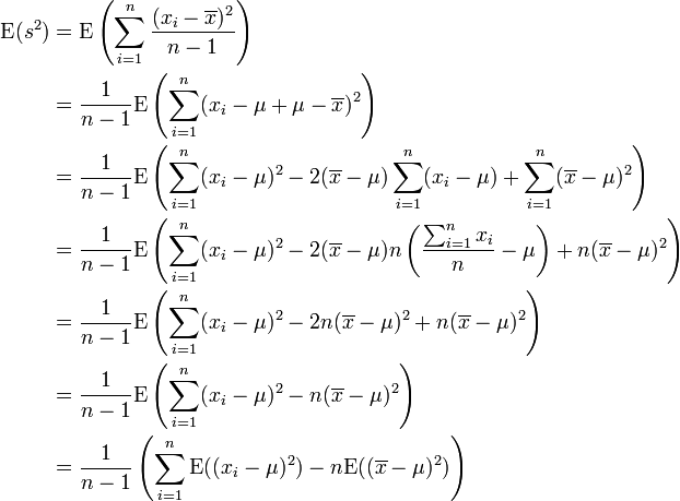
Note that, since x₁, x₂, · · · , x_n are a random sample from a distribution with variance ?², it follows that for each i = 1, 2, . . . , n:

$\operatorname{E}((x_i-\mu)^2) = \sigma^2 \, ,$

Wackerly, D., Mendenhall, W., & Scheaffer, R. L. (2001), p.372

and also

$\operatorname{Var}(\overline{x}) = \operatorname{E}((\overline{x}-\mu)^2) = \sigma^2/n. \,$

This is a property of the variance of uncorrelated variables, arising from the Bienaymé formula. For a proof, see here. The required result is then obtained by substituting these two formulae:

$\operatorname{E}(s^2) = \frac{1}{n-1}\left[\sum_{i=1}^n \sigma^2 - n(\sigma^2/n)\right] = \frac{1}{n-1}(n\sigma^2-\sigma^2) = \sigma^2. \,$

because of Functional invariance of MLE, if g(?) is any transformation of ?, then the MLE for ? = g(?) is by definition

$\widehat{\alpha} = g(\,\widehat{\theta}\,). \,$

thefore it can be shown that the MLE of standard deviation is the square root of

$\widehat\sigma^2 = \sum_{i=1}^n(x_i-\widehat{\mu})^2/n.$

Devore, P. J. L. (2007), p. 249

not the The most common measure used is the sample standard deviation, which is defined by

$s = \sqrt{\frac{1}{n-1} \sum_{i=1}^n (x_i - \overline{x})^2}\,,$

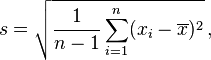
where $\{x_1,x_2,\ldots,x_n\}$ is the sample (formally, realizations from a random variable X) and $\overline{x}$ is the sample mean.

This is also a a biased estimator for standard deviation.The square root is a nonlinear function, and only linear functions commute with taking the expectation. Since the square root is a concave function, it follows from Jensen’s inequality that the square root of the sample variance is an underestimate. The use of n ? 1 instead of n in the formula for the sample variance is known as Bessel’s correction, which corrects the bias in the estimation of the sample variance, and some, but not all of the bias in the estimation of the sample standard deviation.

The unbiased estimation for standard deviation is:

http://en.wikipedia.org/wiki/Unbiased_estimation_of_standard_deviation

====================================================================

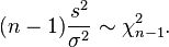
Distribution of the sample varianceBeing a function of random variables, the sample variance is itself a random variable, and it is natural to study its distribution. In the case that y_i are independent observations from a normal distribution, Cochran’s theorem shows that s² follows a scaled chi-square distribution:

$(n-1)\frac{s^2}{\sigma^2}\sim\chi^2_{n-1}.$

As a direct consequence, it follows that E(s²) = ?²

The Variance of sample variance will be (2*df) which will be 2*(n-1)

If the y_i are independent and identically distributed, but not necessarily normally distributed, then

$\operatorname{E}[s^2] = \sigma^2, \quad \operatorname{Var}[s^2] = \sigma^4 \left( \frac{2}{n-1} + \frac{\kappa}{n} \right),$

where ? is the kurtosis of the distribution. If the conditions of the law of large numbers hold, s² is a consistent estimator of ?².

Devore, J. L. (2008). Probability and Statistics for Engineering and the Sciences, Enhanced Review Edition (7th ed.). Duxbury Press.

Devore, P. J. L. (2007). Student Solutions Manual for Devore’s Probability and Statistics for Engineering and the Sciences, 7th (7th ed.). Duxbury Press.

Johnson, R. A., & Wichern, D. W. (2007). Applied Multivariate Statistical Analysis (6th ed.). Prentice Hall.

Wackerly, D., Mendenhall, W., & Scheaffer, R. L. (2001). Mathematical Statistics with Applications (6th ed.). Duxbury Press.

Demosophy.org

Estimators for a population’s parameters

Comments

Estimators for a population’s parameters — No Comments

Leave a Reply