
[mathjax]

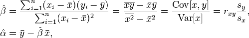
Pearson’s R is based on the standardized distance of x and y from Xbar and Ybar.
![]()
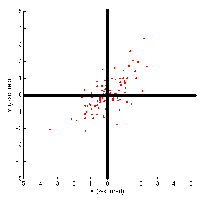
Points in first and third quadrants result in positive contributions and points in second and fourth quadrants lead to negative contribution to r.
But because average is not meaningful for ordinal data, the measures of ordinal associations are based on concordance between all possible pairs.

r will be equal to the slope of the regression line when the dispersion of of Y and X is the same.
in other words
If we standardize Y and X, and chart the observations based on the number of standard devisions, the (x,y) are the number of standard deviations away from 0. In this situation the r is the slope.
r=b*(Sx/Sy)
r is the slope of regression line of standardized y and x.
For a non-standardized regression line r will be low if Sy is big (when Ys have a lot of dispersion)
============================================

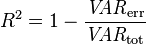
r is not an unbiased estimate of ρ. A relatively unbiased estimate is the adjusted correlation coefficient :


Adjusted R2 is

where p is the total number of regressors in the linear model (not counting the constant term), and n is the sample size.
Adjusted R2 can also be written as

where dft is the degrees of freedom n– 1 of the estimate of the population variance of the dependent variable, and dfe is the degrees of freedom n – p – 1 of the estimate of the underlying population error variance.
The principle behind the adjusted R2 statistic can be seen by rewriting the ordinary R2 as
| Assumption | Problem | Test | Solution |
| Predictors are Independent | Multicollinearity | Tolerance, VIF | Drop Variables, Mean Center, Combine variables into index |
| Errors are statistically independent | autocollinearity | Durbin-Watson Test, plot residuals over time | Adjust data |
| Distribution of residuals is normal, random | heteroscedasticity, nonlinearity |
plot residuals against predicted y, quantile comparison plot, graph residuals in a boxplot, histogram | transform y and/or x |
| Errors are not “unusual” (outliers) | large outliers, influential points | quantile comparion plot, test leverage and influence, Cook’s Distance, added variable plots, graph studentized residuals vs. predicted y | remove outliers |
| Linear relationship is the correct function | non-linear relationship | added-variable plot, component and residual plot | transform predictors, add terms |
From: https://www2.bc.edu/~stevenw/MB875/mb875_RegDiag.htm
R (packages gee, geepack and multgee) are for Generalized estimating equation GEE
A generalized estimating equation (GEE) is used to estimate the parameters of a generalized linear model with a possible unknown correlation between outcomes.
Parameter estimates from the GEE are consistent even when the covariance structure is misspecified, under mild regularity conditions.
The focus of the GEE is on estimating the average response over the population (“population-averaged” effects) rather than the regression parameters that would enable prediction of the effect of changing one or more covariates on a given individual.
GEEs are usually used in conjunction with Huber-White standard error estimates, also known as “robust standard error” or “sandwich variance” estimates.
In the case of a linear model with a working independence variance structure, these are known as “heteroskedasticity consistent standard error” estimators.
GEE unified several independent formulations of these standard error estimators in a general framework.
GEEs belong to a class of semiparametric regression techniques because they rely on specification of only the first two moments.
Under correct model specification and mild regularity conditions, parameter estimates from GEEs are consistent.
They are a popular alternative to the likelihood–based generalized linear mixed model which is more sensitive to variance structure specification.
They are commonly used in large epidemiological studies, especially multi-site cohort studies because they can handle many types of unmeasured dependence between outcomes.
http://en.wikipedia.org/wiki/Generalized_estimating_equation
====================================================
multinomial association cran – Google Search
An R Package for Hierarchical Multinomial Marginal Models
Package ‘multgee’ Marginal Models For Correlated Ordinal Multinomial Responses
Package ‘MultinomialCI’
Package ‘CoinMinD’ Simultaneous Confidence Interval for Multinomial Proportion
———————————–
Tests of independence / dependence
coin: A Computational Framework for Conditional Inference
oneway_test two- and K-sample permutation test
wilcox_test Wilcoxon-Mann-Whitney rank sum test ( tests for ordered categorical data)
normal_test van der Waerden normal quantile test
median_test Median test
kruskal_test Kruskal-Wallis test
ansari_test Ansari-Bradley test
fligner_test Fligner-Killeen test
chisq_test Pearson’s χ 2 test
cmh_test Cochran-Mantel-Haenszel test (Independence in general two- or three-dimensional contingency tables can be tested)
lbl_test linear-by-linear association test ( tests for ordered categorical data)
surv_test two- and K-sample logrank test ( tests for ordered categorical data)
maxstat_test maximally selected statistics
spearman_test Spearman’s test
friedman_test Friedman test
wilcoxsign_test Wilcoxon-Signed-Rank test ( tests for ordered categorical data)
mh_test marginal homogeneity test (Maxwell-Stuart).
coin: A Computational Framework for Conditional Inference
Package ‘coin’
Chapter Conditional Inference
Order-restricted Scores Test for the Evaluation of Population …
Exact tests
In statistics, an exact (significance) test is a test where all assumptions, upon which the derivation of the distribution of the test statistic is based, are met as opposed to an approximate test (in which the approximation may be made as close as desired by making the sample size big enough). This will result in a significance test that will have a false rejection rate always equal to the significance level of the test. For example an exact test at significance level 5% will in the long run reject true null hypotheses exactly 5% of the time.
So when the result of a statistical analysis is said to be an “exact test” or an “exact p-value”, it ought to imply that the test is defined without parametric assumptions and evaluated without using approximate algorithms.
http://en.wikipedia.org/wiki/Exact_test
http://mathworld.wolfram.com/FishersExactTest.html
http://en.wikipedia.org/wiki/Fisher%27s_exact_test
http://en.wikipedia.org/wiki/Barnard%27s_test
Implementation of Barnard’s exact test using R
http://www.statmethods.net/stats/resampling.html
FisherExactCalculation.pdf
Package ‘Exact’ – Cran Unconditional exact tests for 2×2 contingency tables
Package ‘Barnard’ implements the barnardw.test function for performing Barnard’s unconditional test of superiority. This is a more powerful alternative of Fisher’s exact test for 2×2 contingency tables.
http://www.r-statistics.com/2010/02/barnards-exact-test-a-powerful-alternative-for-fishers-exact-test-implemented-in-r/
Calculators:
Freeman-Halton extension of Fisher’s exact test to compute the (two-tailed) probability of obtaining a distribution of values in a 3×3 contingency table, given the number of observations in each cell.
http://www.danielsoper.com/statcalc3/calc.aspx?id=59
http://vassarstats.net/fisher3x3.html
http://vassarstats.net/index.html
http://in-silico.net/tools/statistics/fisher_exact_test
—————
jonckheere.test
Exact/permutation version of Jonckheere-Terpstra test (Jonckheere-Terpstra test to test for ordered differences among classes)
R Package ‘clinfun’
http://en.wikipedia.org/wiki/Jonckheere%27s_trend_test
—————
Non-parametric tests
http://en.wikipedia.org/wiki/Nonparametric_statistics
———————
gMWT-package
Implementations of Generalized Mann-Whitney Type Tests
The package provides nonparametric tools for the comparison of several groups/treatments when
the number of variables is large. The tools are the following.
Package ‘gMWT’
—————————-
Exact statistics
http://en.wikipedia.org/wiki/Exact_statistics
—————————————–
The formulae for confidence interval:

and prediction interval:
|

Confidence interval is an estimate of an interval in which mean of observations will fall when x=xi
In its formula

Tends to 0.
Prediction interval is an estimate of an interval in which future individual observations will fall when x=xi
In its formula

tends to 1
That means that the confidence interval for the mean of the outcomes at xi gets smaller as sample size grows. (as Central limit Theorem would suggest) which means that by increase of the sample size our estimate for the average (mean) outcome for xi gets better.

But the dispersion of the distribution of y|xi “the probability of an individual outcome” at xi, Doesn’t change very much because central limit theorem is related to central tendencies not to individual behavior or outcomes. Therefore the prediction interval doesn’t change very much.
Individual behavior remains uncertain no matter how much you increase your sample size 😉

![]()