
Center of gravity C in physics is where sum of all moments which is mass x distance (md) is zero
where m s are masses in the system
Moment of inertia which is more when the masses are farther from C is
Moment of inertia is an object’s resistance to changes in its rotation rate around a specific axis. It is the rotational equivalent of mass in linear motion. A higher moment of inertia means it takes more torque to start, stop, or change an object’s spinning motion
Torque ( ): The rotational version of Newton’s second law (
 ) is
) is  , where
  is angular acceleration.
Angular Momentum ( ): This quantity, which remains constant unless an external torque acts, is
  .
.
 and
and  with initial velocities
  and
and  , the final velocities
  and
and  are found:
1. Define Conservation Laws
- Conservation of Momentum:

- Conservation of Kinetic Energy:

2. Rearrange and Factor
- Momentum:

- Energy:

 , the energy equation becomes:
 ![\[m_1(v_1 - v_{1f})(v_1 + v_{1f}) = m_2(v_{2f} - v_2)(v_{2f} + v_2)\]](https://demosophy.org/wp-content/ql-cache/quicklatex.com-0640599de39d1b9f018bc30f1f901678_l3.png "Rendered by QuickLaTeX.com")
3. Simplify Using Ratio
![\[\frac{m_1(v_1 - v_{1f})(v_1 + v_{1f})}{m_1(v_1 - v_{1f})} = \frac{m_2(v_{2f} - v_2)(v_{2f} + v_2)}{m_2(v_{2f} - v_2)}\]](https://demosophy.org/wp-content/ql-cache/quicklatex.com-6eaae59f6aaf9a78e55aca0cab6b64cf_l3.png "Rendered by QuickLaTeX.com")
![\[v_1 + v_{1f} = v_2 + v_{2f}\]](https://demosophy.org/wp-content/ql-cache/quicklatex.com-764614cbd6bcc5d4f59f1c90757d5823_l3.png "Rendered by QuickLaTeX.com")
This yields the Relative Velocity Relationship:
 , meaning the velocity of approach equals the velocity of recession.
4. Substitute and Solve
from the relative velocity equation:  . Substitute this back into the original momentum equation:
 ![\[m_1v_1 + m_2v_2 = m_1v_{1f} + m_2(v_1 - v_2 + v_{1f})\]](https://demosophy.org/wp-content/ql-cache/quicklatex.com-e0342f1d0d110456d49e079c3f358c68_l3.png "Rendered by QuickLaTeX.com")
Solving for
gives the first final velocity formula. A similar substitution for yields the formula for .✅ Final Velocities
![\[v_{1f} = \frac{(m_1 - m_2)v_1 + 2m_2v_2}{m_1 + m_2}\]](https://demosophy.org/wp-content/ql-cache/quicklatex.com-e8dfa3b2ef63c4582ca83929fe4bcf0c_l3.png "Rendered by QuickLaTeX.com")
![\[v_{2f} = \frac{(m_2 - m_1)v_2 + 2m_1v_1}{m_1 + m_2}\]](https://demosophy.org/wp-content/ql-cache/quicklatex.com-52451eadaa3c456fc5ee37d9782625aa_l3.png "Rendered by QuickLaTeX.com")
========================================================================
In statistics we call
and we know that 
Therefore mean is like center of gravity.
and f(x)x is called the first moment of each x, and sum of the moments around mean is zero.
As sum of the moments of masses composing a matter around the center of gravity is zero.
We define
For a variable such as Z for which mu is zero
The second moment is is not Zero and is more when the observations are more dispersed similar to Moment of inertia which is more when the masses are farther from Center of gravity.
===================================================
Consider function M(t)
since

M(t)=\int (1+tx+\frac{t^2x^2}{2!}+\frac{t^3}{3!}…)f(x) dx
Therefore we call M(t) moment generating function 🙂
https://onlinecourses.science.psu.edu/stat414/node/73
=-=-=-=-=-=-=-=-=-
The moment generating function (MGF) is equivalent to the two-sided Laplace transform of the probability density function (PDF) evaluated at (-t)
The Laplace transform is a mathematical tool that converts a function of time, f(t), into a function of complex frequency, F(s).
 -domain measures both oscillations and growth or decay.
s=sigma +j*omega
- Sigma: Represents damping or growth/decay. It dictates how fast a signal dies out or blows up over time.
- Omega: Represents angular frequency 2*pi*f. It dictates how fast the signal oscillates.


 into the Laplace transform of a probability density function (PDF), you get the MGF:
 ![M_X(t) = E[e^{tX}]](https://demosophy.org/wp-content/ql-cache/quicklatex.com-b608f6b97662ad6c18c1c3fcd553b253_l3.png "Rendered by QuickLaTeX.com") .
.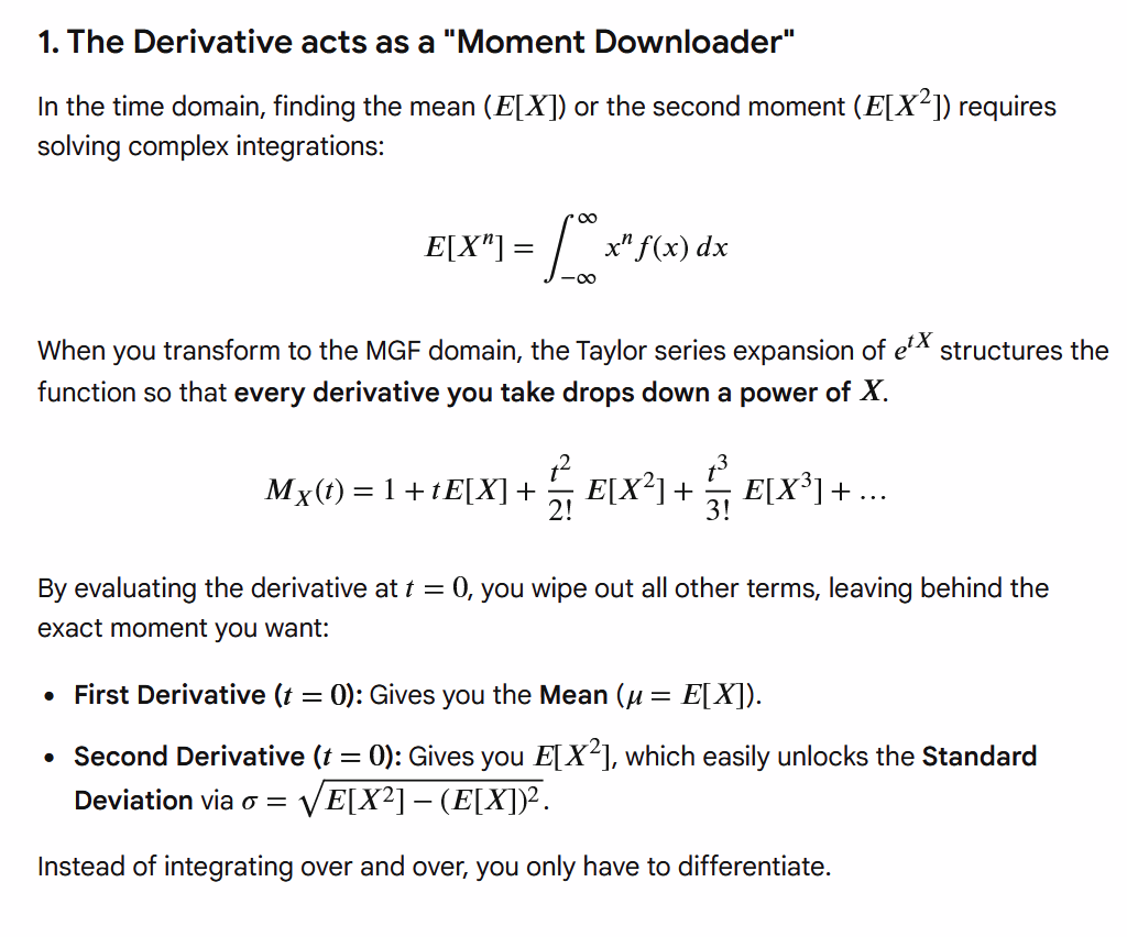
1. The Derivative acts as a “Moment Downloader”
![E[X]](https://demosophy.org/wp-content/ql-cache/quicklatex.com-4249815a79caf7890371efa1a609bb7f_l3.png "Rendered by QuickLaTeX.com") ) or the second moment (
) or the second moment (![E[X^2]](https://demosophy.org/wp-content/ql-cache/quicklatex.com-d4ed6d18fd14734e28e532b101ed5a87_l3.png "Rendered by QuickLaTeX.com") ) requires solving complex integrations:
) requires solving complex integrations: ![\[E[X^n] = \int_{-\infty}^{\infty} x^n f(x) \, dx\]](https://demosophy.org/wp-content/ql-cache/quicklatex.com-44bb65060903eab0757a73fc43d387d6_l3.png "Rendered by QuickLaTeX.com")
 structures the function so that every derivative you take drops down a power of
  .
. ![\[M_X(t) = 1 + tE[X] + \frac{t^2}{2!}E[X^2] + \frac{t^3}{3!}E[X^3] + \dots\]](https://demosophy.org/wp-content/ql-cache/quicklatex.com-b7b401c575b1dc41dd41b488860c4928_l3.png "Rendered by QuickLaTeX.com")
 , you wipe out all other terms, leaving behind the exact moment you want:
- First Derivative (
 ): Gives you the Mean (
![\mu = E[X]](https://demosophy.org/wp-content/ql-cache/quicklatex.com-f4fff185454ab9f79ea26d352a6960cb_l3.png "Rendered by QuickLaTeX.com") ).
). - Second Derivative (): Gives you , which easily unlocks the Standard Deviation via
![\sigma = \sqrt{E[X^2] - (E[X])^2}](https://demosophy.org/wp-content/ql-cache/quicklatex.com-50150643b7e4240381d5309b885f0a86_l3.png "Rendered by QuickLaTeX.com") .
.

2. Convolution Becomes Simple Multiplication
 ).
).- In the Time/Probability Domain: To find the probability distribution of
 , you must solve a highly complex calculus operation called convolution:

- In the Frequency/MGF Domain: Convolution completely unravels. The transformation maps addition in the time domain directly to basic multiplication in the frequency domain:

3. Summary: Why it Works
- Do you have a specific distribution (like the Normal, Exponential, or Binomial) you want to derive the mean for?
- Would you like to see the step-by-step math for proving the sum of two variables using this trick?


