Statistics - Demosophy.org

An experiment is a planned operation carried out under controlled conditions.

Outcome is a possible result of a random experiment. it is an element of a sample space.

Sample space is the set of all possible outcomes.

Event is a set of some of the possible outcomes; a subset of the sample space, that may be interesting.

==================================================

Mediator is …

Control variable is an independent variable that its effect size is studied as part of the research and is not in the hypotheses but its existence may have impact over Dependent Variable (DV) and therefore it is included in the model and is kept under control or “constant” to minimize the impact on the relationships between IVs & DV.

Moderating variable is a variable that is being studied to evaluate how it influences the relationship between the independent and dependent variables. Moderating variable is usually explicitly stated as part of the hypothesis. The effect size between dependent and independent variables is a function of moderator variable.

================================================

A complete set of proofs by Jennifer L. Loveland:

http://digitalcommons.usu.edu/gradreports/14/

Courses on statistics with mathematical proof

http://ocw.mit.edu/courses/mathematics/18-443-statistics-for-applications-fall-2006/lecture-notes/ (best no video)

http://www.stat.ucla.edu/~nchristo/statistics100B/ ( no video)

——

OCW scholar edition ! ?

http://ocw.mit.edu/courses/electrical-engineering-and-computer-science/6-041sc-probabilistic-systems-analysis-and-applied-probability-fall-2013/index.htm (video)

play list https://www.youtube.com/watch?v=j9WZyLZCBzs&index=1&list=PLUl4u3cNGP61MdtwGTqZA0MreSaDybji8

——

https://onlinecourses.science.psu.edu/stat414/( good course no video)

=============================================

Distributions with proof of theorems http://www.statlect.com/distri.htm

Good arguments for interesting topics

http://core.ecu.edu/psyc/wuenschk/StatsLessons.htm

NCSSM Statistics Leadership Institute Notes

http://courses.ncssm.edu/math/Stat_Inst/Notes.htm

http://courses.ncssm.edu/math/Stat_Inst/Stats2007/2007_statistics_institute.htm

https://www.youtube.com/watch?v=FUmTji5qRJM https://www.youtube.com/watch?v=cC19I3vRlIo https://www.youtube.com/watch?v=vDXEo2vzKbQ

=============================================================

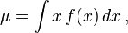
Moments The center of mass $\mathbf{R}$ of a system of particles of total mass $M$ is defined as the average of their positions, $\mathbf{r}_i$ , weighted by their masses, $m_i$ :^[3]

$\mathbf{R} = \frac{1}{M} \sum m_i \mathbf{r}_i.$

For a continuous distribution with mass density $\rho(\mathbf{r})$ , the sum becomes an integral:^[4]

$\mathbf R =\frac 1M \int \mathbf{r} \; dm = \frac 1M \int\rho(\mathbf{r})\, \mathbf{r} \ dV.$

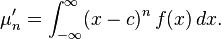
Definition of the center of gravity is the point around which all of the torques or first moments is zero. === In mathematics, a moment is,a quantitative measure of the shape of a set of points. Other moments describe other aspects of a distribution such as how the distribution is skewed from its mean, or peaked. The mathematical concept is closely related to the concept of moment in physics, The n^th moment of a real-valued continuous function f(x) of a real variable about a value c is

$\mu'_n=\int_{-\infty}^\infty (x - c)^n\,f(x)\,dx.\,\!$

therefore the first moment around center of gravity is zero.

The first moment is a weighted average of distance of mass from center, it is a measure of central tendency.

In probability theory, the expected value (or expectation, or mathematical expectation, or mean, or the first moment) of a random variable is the weighted average of all possible values that this random variable can take on.

If the probability distribution of X admits a probability density function f(x), then the expected value can be computed as

$ \operatorname{E}[X] = \int_{-\infty}^\infty x f(x)\, \operatorname{d}x . $

if f is the gravitational force, and x is the distance of a mass from center of gravity, the E(X) will be Zero.

========================

The moment of inertia of an object about a given axis describes how difficult it is to change its angular motion about that axis. Therefore, it encompasses not just how much mass the object has overall, but how far each bit of mass is from the axis. The further out the object’s mass is, the more rotational inertia the object has, and the more rotational force (torque, the force multiplied by its distance from the axis of rotation) is required to change its rotation rate. In this expression the quantity in parentheses is called the moment of inertia of the body (with respect to the specified axis of rotation). It is a purely geometric characteristic of the object, as it depends only on its shape and the position of the rotation axis. The moment of inertia is usually denoted with the capital letter I:

$ I = \sum_{i=1}^N m_i r_i^2\ . $

It is worth emphasizing that r_i here is the distance from a point to the axis of rotation, not to the origin. As such, the moment of inertia will be different when considering rotations about different axes. Similarly, the moment of inertia of a continuous solid body rotating about a known axis can be calculated by replacing the summation with the integral:

$ I = \int_V \rho(\mathbf{r})\,d(\mathbf{r})^2 \, \mathrm{d}V\!(\mathbf{r}), $

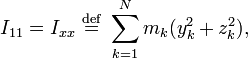
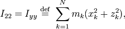
where r is the radius vector of a point within the body, ?(r) is the mass density at point r, and d(r) is the distance from point r to the axis of rotation. The integration is evaluated over the volume V of the body. In three dimensions, if the axis of rotation is not given, we need to be able to generalize the scalar moment of inertia to a quantity that allows us to compute a moment of inertia about arbitrary axes. This quantity is known as the moment of inertia tensor For a rigid object of $N$ point masses $m_{k}$ , the moment of inertia tensor (with respect to the origin) has components given by

$ \mathbf{I} = \begin{bmatrix} I_{11} & I_{12} & I_{13} \\ I_{21} & I_{22} & I_{23} \\ I_{31} & I_{32} & I_{33} \end{bmatrix} $ ,

where

$I_{11} = I_{xx} \ \stackrel{\mathrm{def}}{=}\ \sum_{k=1}^{N} m_{k} (y_{k}^{2}+z_{k}^{2}),\,\!$

$I_{22} = I_{yy} \ \stackrel{\mathrm{def}}{=}\ \sum_{k=1}^{N} m_{k} (x_{k}^{2}+z_{k}^{2}),\,\!$

$I_{33} = I_{zz} \ \stackrel{\mathrm{def}}{=}\ \sum_{k=1}^{N} m_{k} (x_{k}^{2}+y_{k}^{2}),\,\!$

$I_{12} = I_{xy} \ \stackrel{\mathrm{def}}{=}\ -\sum_{k=1}^{N} m_{k} x_{k} y_{k},\,\!$

$I_{13} = I_{xz} \ \stackrel{\mathrm{def}}{=}\ -\sum_{k=1}^{N} m_{k} x_{k} z_{k},\,\!$

$I_{23} = I_{yz} \ \stackrel{\mathrm{def}}{=}\ -\sum_{k=1}^{N} m_{k} y_{k} z_{k},\,\!$

and $I_{12}=I_{21}$ , $I_{13}=I_{31}$ , and $I_{23}=I_{32}$ . (Thus $I$ is a symmetric tensor.) Note that the scalars $I_{ij}$ with $i\ne j$ are called the products of inertia. Here $I_{xx}$ denotes the moment of inertia around the $x$ -axis when the objects are rotated around the x-axis, $I_{xy}$ denotes the moment of inertia around the $y$ -axis when the objects are rotated around the $x$ -axis, and so on. The moment of inertia tensor about the center of mass of a 3-dimensional rigid body is related to the covariance matrix of a trivariate random vector whose probability density function is proportional to the pointwise density of the rigid body. The variance of a real-valued random variable is its second central moment which is a measure of dispersion around the mean. If the random variable X is continuous with probability density function f(x), then the variance equals the second central moment around mean, given by

$\operatorname{Var}(X) =\int (x-\mu)^2 \, f(x) \, dx\,,$

where $\mu$ is the expected value,

$\mu = \int x \, f(x) \, dx\,,$

and where the integrals are definite integrals taken for x ranging over the range of X. ==============================================================

The variance of a sum of two random variables is given by: $\sigma ^{2}(ax+by)=a^{2}\sigma _{a}^{2}+b^2\sigma_{b}^{2}+2abCov(x,y)$ Product of independent variables If two variables X and Y are independent, the variance of their product is given by: $\sigma ^{2}(xy)=\mu_x\sigma _y^{2}+\mu_y^2\sigma_x^{2}+\sigma _x^{2}\sigma _y^{2}$

Statistics in SQL

Directional statistics

https://en.wikipedia.org/wiki/Directional_statistics

Since 11 April 2023: 303 total views, 1 views today