In mathematics, an autonomous system or autonomous differential equation is a system of ordinary differential equations which does not explicitly depend on the independent variable. When the variable is the time, they are also named Time-invariant system.

A time-invariant (TIV) system is one whose output does not depend explicitly on time.

Many systems, the time dependence “averages out” over the time scales being considered. (Blanchard, 2005, p.76)

Blanchard, P., Devaney, R. L., & Hall, G. R. (2005). Differential Equations (3rd ed.). Brooks Cole.

If the input signal $x(t)$ produces an output $y(t)$ then any time shifted input, $x(t + \delta)$ , results in a time-shifted output $y(t + \delta)$

This property can be satisfied if the transfer function of the system is not a function of time except expressed by the input and output.

An autonomous differential equation is one where there is no explicit occurrence of the independent variable.

Many laws in physics, where the independent variable is usually assumed to be time, are expressed as autonomous systems because it is assumed the laws of nature which hold now are identical to those for any point in the past or future.

Autonomous systems are closely related to dynamical systems. Any autonomous system can be transformed into a dynamical system and, using very weak assumptions, a dynamical system can be transformed into an autonomous system.

==========================================================

Linear Differential Equations

A linear differential equation is any differential equation that can be written in the following form.

The important thing to note about linear differential equations is that there are no products of the function,, and its derivatives and neither the function or its derivatives occur to any power other than the first power.

The coefficients and can be zero or non-zero functions, constant or non-constant functions, linear or non-linear functions. Only the function,, and its derivatives are used in determining if a differential equation is linear.

=============================================================

A second-order linear differential equation has the form
equations of this type arise in the study of the motion of a spring. In Additional Topics: Applications of
Second-Order Differential Equations we will further pursue this application as well as the
application to electric circuits.

Such equations are called homogeneous linear equations. Thus, the form of a second-order linear
homogeneous differential equation is

=====================================

Homogeneous: A differential equation is homogeneous if every single term contains the dependent variables or their derivatives.

One is that a first-order ordinary differential equation is homogeneous (of degree 0) if it has the form

$\frac{dy}{dx} = F(x,y)$

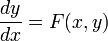
where x is an independent variable, y a dependent variable, and F(x, y) is a homogeneous function of degree n; in other words scalar multiplying each variable by a constant ? leaves the function unchanged:

$F(\lambda x,\lambda y) = \lambda^n F(x,y)$ .

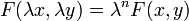In a more general form:

$N(x,y)\,dx + M(x,y)\,dy = 0$

where M and N are also homogeneous.

========================================================================

A linear non-homogeneous ordinary differential equation with constant coefficients has the general form of

where are all constants and .

second-order nonhomogeneous linear differential equations
with constant coefficients, that is, equations of the form

where , , and are constants and is a continuous function. The related homogeneous
equation

=============================================================

Laplace transform cannot be used to solve nonlinear differential equation easily.

Laplace transform can be used to solve linear but even non-homogenous, non-autonomous differential equations

===============================================================.

A system in which the (laplace transform of impulse response) system function or transfer function considering initial state is such that

when s->0 the bounds of result is limited and approaches Ya, will have the same result for any input because H(s)=Y(s)/X(s).

the system has an attractor or sink equilibrium point Ya in phase plane or slope plane at that value when x->infinity. which means the system has a stable steady state.

Laplace transform properties and proof of final value theorem

where is Laplace transform coming from

Application of Laplace Transforms in Control

stability

Controllers

————————————————

State variable method is a fundamental method because it relies on the diff equations.

It deals with first order diffs .

A state space representation is a mathematical model of a system with memory as a set of input, output and state variables related by first-order differential equations. To abstract from the number of inputs, outputs and states, the variables are expressed as vectors.

State is a variable for which we have a first order differential equation.

The internal state variables are the smallest possible subset of system variables that can represent the entire state of the system at any given time. The minimum number of state variables required to represent a given system, $n$ , is usually equal to the order of the system’s defining differential equation. If the system is represented in transfer function form, the minimum number of state variables is equal to the order of the transfer function’s denominator after it has been reduced to a proper fraction. It is important to understand that converting a state space realization to a transfer function form may lose some internal information about the system, and may provide a description of a system which is stable, when the state-space realization is unstable at certain points.

In electric circuits, the number of state variables is often, though not always, the same as the number of energy storage elements in the circuit such as capacitors and inductors. The state variables defined must be linearly independent; no state variable can be written as a linear combination of the other state variables or the system will not be able to be solved.

Amir: so the number of independent memories determine the number of state variables.

$\dot{\mathbf{x}}(t) = A(t) \mathbf{x}(t) + B(t) \mathbf{u}(t)$

$\mathbf{y}(t) = C(t) \mathbf{x}(t) + D(t) \mathbf{u}(t)$

File:Typical State Space model.png

$\dot{\mathbf{x}}(t) = A(t) \mathbf{x}(t) + B(t) \mathbf{u}(t)$

$\mathbf{y}(t) = C(t) \mathbf{x}(t) + D(t) \mathbf{u}(t)$

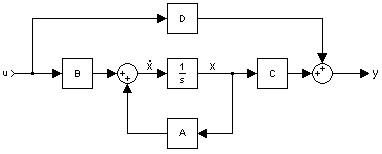
State Space representation State Space

State Space Video State Space Video Utah Modeling Systems in State-Space Form Utah

Utah State Space Course

State Space Circuit Analysis India

——————————————————————————-

Control with Matlab

Linear Dynamical systems

http://lpsa.swarthmore.edu/LaplaceXform/FwdLaplace/LaplaceProps.html#Second_

First order differential equation

Taking the Laplace Transform of the eqn		where y(0) represents the initial conditions

Solves for Y(s)

so that

A standard second order transfer function model (with u as input variable
and y as output variable) is

where K is the gain, (zeta) [dimension 1] is the relative damping factor,
and Omega [rad/s] is the undamped resonance frequency.

Laplace and Fourier

Stability, Zeros, Poles

The step response is the integral (w.r.t time) of the impulse response.
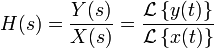
The transfer function is the Laplace transform of the impulse response.

also
$H(s) = \frac{Y(s)}{X(s)} = \frac{ \mathcal{L}\left\{y(t)\right\} }{ \mathcal{L}\left\{x(t)\right\} }$

If a system is represented by a single n^thorder differential equation, it is easy to represent it in transfer function form. Starting with a third order differential equation with x(t) as input and y(t) as output.

To find the transfer function, first take the Laplace Transform of the differential equation (with zero initial conditions). Recall that differentiation in the time domain is equivalent to multiplication by “s” in the Laplace domain.

The transfer function is then the ratio of output to input and is often called H(s).

Impulse responses, step responses and transfer functions

Stability and Pole Locations

Convolution:

https://maxwell.ict.griffith.edu.au/spl/Excalibar/Jtg/Conv.html

http://www.jhu.edu/signals/convolve/

http://www.isip.piconepress.com/projects/speech/software/demonstrations/applets/util/convolution/current/

http://mathlets.org/mathlets/

Oppenheim, A. V., Willsky, A. S., & Hamid, with S. (1996). Signals and Systems (2nd ed.). Prentice Hall.

As explained by oppenheim (1996,p.41) any model used is describing or analyzing a system represents and idealization of that system and any resulting analysis is only as good as the model itself. (Oppenheim, 1996, p.41)

while the concept of memory in a system would suggest storing past input and output values. Although it seems unnatural, in an important group of systems, the current outputs is dependent on the future values of the input and output. (Oppenheim, 1996, p.45)

A system is causal if the output at anytime depends on values of the input at only the present and the past. All memoryless systems are causal.

However, causality is not often essential in applications in which the independent variable is not time.

The following system is causal:

$y(t)=x(t)cos(t+1))$ be\ it depends on x at t and is not anticipating x in future.

(Oppenheim, 1996, p.46-47)

If an LTI system is causal, then the ROC of is a right-sided half plane. In particular, If is rational , then the system is causal if and only if its ROC is the right-sided half plane to the right of the rightmost pole, and the order of numerator is no greater than that of the denominator , so that the ROC is a right-sided plane without any poles

Example of non-causal (acausal) systems

For coefficients of t

$y \left( t \right) =x(at)$

Examples of anti-causal systems

Time reversal

$y \left( t \right) =x(-t)$

wikipedia : http://en.wikipedia.org/wiki/Causal_system

===================================

A stable system is one in which small inputs lead to responses that do not diverge.

(this means a limited input does not create an output that goes beyond any threshold)

Stability of physical systems generally results from the presence of mechanisms that dissipate energy.

If we suppose a system is unstable, then a useful strategy to verify this is to look for a specific bounded input that leads to an unbounded output.

(Oppenheim, 1996, p.49)

An LTI system is stable if and only if its impulse response is absolutely integrable, i.e., the frequency response function $H(j\omega)$ exists, i.e., the ROC of its transfer function contains $j\omega$ -axis:

A causal LTI system with a rational transfer function is stable if and only if all poles of are in the left half of the s-plane, i.e., the real parts of all poles are negative:

Example 1: The transfer function of an LTI is

$\begin{displaymath}H(s)=\frac{1}{a+s} \end{displaymath}$

As shown before, without specifying the ROC, this could be the Laplace transform of one of the two possible time signals .


	$j\omega$ -axis inside ROC	$j\omega$ -axis outside ROC,
$h(t)=e^{-at}u(t)$	causal, stable	causal, unstable

Feedback can be used to stabilize a non-stable system or destabilize a stable system.

A system is time invariant if the behavior and characteristics of the system are fixed over time (Oppenheim, 1996, p.50)

Amir: This means that is doesn’t matter when you apply a signal to the system. If you apply a signal x at t1 and get a response y at t1+d , If you apply a signal x at t2, you will get a response y at t2+d

A linear system is a system that possesses the important property of superposition. if the input is the weighted sum of several signals, the output will be the weighted sum of the responses to those signals. (Oppenheim, 1996, p.53)

A system can be linear and not time invariant. A system can be time invariant and not linear. (Oppenheim, 1996, p.53)

Y=ax1+bx2 is linear
Y=ax1+bx2+c is not linear because y(0)=c. also x1 leads to ax1+c x2 leads to bx2+c but x1 and x2 doesn’t lead to ax1+bx2+2c
Y=ax1+bx2+c is incrementally linear system because dy=adx1+bdx2

Amir what is the reason for the stability of social systems? The energy dissipation in stable physical system is because of the fields that are binding the particles. In Social systems we have to search for the bonds between social actors.

Amir: Social system are continuous time systems with memory. This memory has been limited and short lived. ICT may increase the capacity and longevity of this memory. This means the response to false stimuli will be slower. This resistance to false stimuli comes from the possibility of compare with past. The individuation reduces this memory.

Social system are time variant but their change over time is slow.

I want to hypothesize that many social systems can be considered time invariant. But they are not linear. may be just because of something like c mentioned above.

So they are only incrementally linear?

====================================================

http://en.wikipedia.org/wiki/LTI_system_theory

The fundamental result in LTI system theory is that any LTI system can be characterized entirely by a single function called the system’s impulse response. The output of the system is simply the convolution of the input to the system with the system’s impulse response. This method of analysis is often called the time domain point-of-view. The same result is true of discrete-time linear shift-invariant systems in which signals are discrete-time samples, and convolution is defined on sequences.

Relationship between the time domain and the frequency domain

Equivalently, any LTI system can be characterized in the frequency domain by the system’s transfer function, which is the Laplace transform of the system’s impulse response (or Z transform in the case of discrete-time systems). As a result of the properties of these transforms, the output of the system in the frequency domain is the product of the transfer function and the transform of the input. In other words, convolution in the time domain is equivalent to multiplication in the frequency domain.

For all LTI systems, the eigenfunctions, and the basis functions of the transforms, are complex exponentials. This is, if the input to a system is the complex waveform $A e^{st}$ for some complex amplitude $A$ and complex frequency $s$ , the output will be some complex constant times the input, say $B e^{st}$ for some new complex amplitude $B$ . The ratio $B/A$ is the transfer function at frequency $s$ .

Because sinusoids are a sum of complex exponentials with complex-conjugate frequencies, if the input to the system is a sinusoid, then the output of the system will also be a sinusoid, perhaps with a different amplitude and a different phase, but always with the same frequency. LTI systems cannot produce frequency components that are not in the input.

LTI system theory is good at describing many important systems. Most LTI systems are considered “easy” to analyze, at least compared to the time-varying and/or nonlinear case. Any system that can be modeled as a linear homogeneous differential equation with constant coefficients is an LTI system. Examples of such systems are electrical circuits made up of resistors, inductors, and capacitors (RLC circuits). Ideal spring–mass–damper systems are also LTI systems, and are mathematically equivalent to RLC circuits.

===========================================================

Unilateral Z-transform

Alternatively, in cases where x[n] is defined only for n ? 0, the single-sided or unilateral Z-transform is defined as

$X(z) = \mathcal{Z}\{x[n]\} = \sum_{n=0}^{\infty} x[n] z^{-n}. \$

In signal processing, this definition can be used to evaluate the Z-transform of the unit impulse response of a discrete-time causal system.

An important example of the unilateral Z-transform is the probability-generating function, where the component $x[n]$ is the probability that a discrete random variable takes the value $n$ , and the function $X(z)$ is usually written as $X(s)$ , in terms of $s = z^{-1}$ . The properties of Z-transforms (below) have useful interpretations in the context of probability theory.

The stability of a system can also be determined by knowing the ROC alone. If the ROC contains the unit circle (i.e., $\left| z \right| = 1\$ ) then the system is stable. In the above systems the causal system (Example 2) is stable because $\left| z \right| > 0.5\$ contains the unit circle.

If you are provided a Z-transform of a system without an ROC (i.e., an ambiguous $x[n]\$ ) you can determine a unique $x[n]\$ provided you desire the following:

Stability
Causality

If you need stability then the ROC must contain the unit circle. If you need a causal system then the ROC must contain infinity and the system function will be a right-sided sequence. If you need an anticausal system then the ROC must contain the origin and the system function will be a left-sided sequence. If you need both, stability and causality, all the poles of the system function must be inside the unit circle.

Relationship to Laplace transform

The Bilinear transform is a useful approximation for converting continuous time filters (represented in Laplace space) into discrete time filters (represented in z space), and vice versa. To do this, you can use the following substitutions in H(s) or H(z):

$\, s =\frac{2}{T} \frac{(z-1)}{(z+1)} \quad$

from Laplace to z (Tustin transformation), or

$\, z =\frac{2+sT}{2-sT} \quad$

from z to Laplace. Through the bilinear transformation, the complex s-plane (of the Laplace transform) is mapped to the complex z-plane (of the z-transform). While this mapping is (necessarily) nonlinear, it is useful in that it maps the entire $j \Omega$ axis of the s-plane onto the unit circle in the z-plane. As such, the Fourier transform (which is the Laplace transform evaluated on the $j \Omega$ axis) becomes the discrete-time Fourier transform. This assumes that the Fourier transform exists; i.e., that the $j \Omega$ axis is in the region of convergence of the Laplace transform.

Oppenheim video

Dynamical Systems

https://archive.org/details/DynamicalSystemModelsAndSymbolicDynamics

Demosophy.org

Signals and systems