Classification tree in R

Classification trees in R

library(rpart)

# Load the iris data that we've been working with
#The response in the iris data is a categorical variable with no particular order, "Species".

data(iris)

# Set the random number seed so that the results
# are the same each time we run the example (if we
# didn't set this the results might differ a bit each time
# because the subsampling process below is stochastic)
set.seed(2568)

Next, we will split our data into training data that we use to fit the model, and test data we use to validate the model. To do this, we will randomly select rows from our dataframe and assign them to the training data. All unsampled rows will be assigned to the test data set.

# Define a variable to subsample rows of the
# iris dataframe
n <- nrow(iris)

# Define a random subsample of the original data.
# We will use these data as a training data set,
# that we will then use to fit the model. The object
# `train` is just a random sample of row numbers from
# the total number of rows ini the iris data.
# Here, we take half the data
train <- sort(sample(1:n, floor(n / 2)))

# We can define separate data frames for the training
# data and the test data using the indices contained
# in `train`.

# Training data
iris.train <- iris[train, ]

# Test data
iris.test <- iris[-train, ]

Then, we can fit the classification tree to the training data.

# Fit the tree
iris_cart <- rpart(Species ~ ., # Formula: '.' means entire dataframe
  data = iris, # Using iris data
  subset = train # More specifically, the training data
)

By default, rpart uses gini impurity to select splits when performing classification. (If you’re unfamiliar read this article.) You can use information gain instead by specifying it in the parms parameter.

 




mytree <- rpart(
  Fraud ~ RearEnd, 
  data = train, 
  method = "class",
  parms = list(split = 'information'), 
  minsplit = 2, 
  minbucket = 1
)

https://www.gormanalysis.com/blog/decision-trees-in-r-using-rpart/


# Install and load the packages library(rattle) # We'll use this one to make some more functional plots library(RColorBrewer) # We'll use this one for colors 

 # Now, make it fancy 
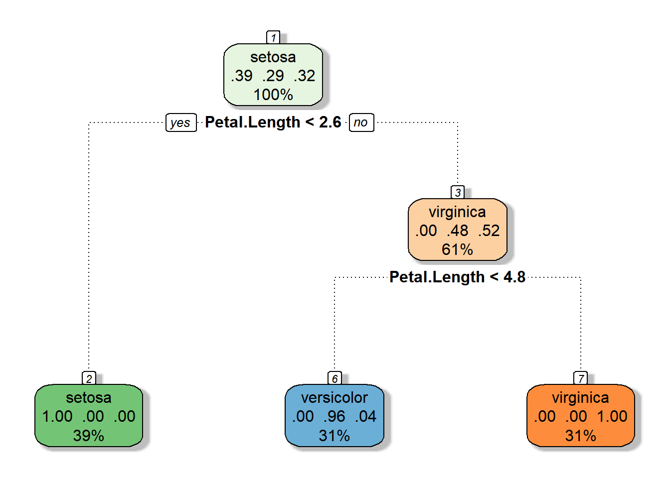
fancyRpartPlot(iris_cart, main = "", sub = "")